Practice Quizzes#
Week 1 - Ballpark estimates#
There are three practice quizzes below, each with three questions. The prompt is the same for all three of them:
Ballpark estimates: For each of the quantities below, come up with a ballpark estimate. Be sure to explain your reasoning and show your work—you will be graded on how you broke up the problem and whether your reasoning made sense, rather than the accuracy of your estimate.
Practice Quiz #1#
How many cups of coffee are consumed on Stanford campus on an average Monday?
How many hours of human labor are spent on hair styling in the US in a year?
How many dice would it take to fill the STATS 60 classroom (room 200-02)?
Practice Quiz #2#
How many Honda Civics could you park on the quad (assuming that none of them are touching)?
How many hours of human labor are spent each year on correcting typos?
How many people in the U.S. have the letter “a” in their first name?
Practice Quiz 3#
How many gallons of milk are consumed in the Bay Area each year?
How long would it take you to empty the fountain in white plaza using only a teaspoon?
How many textbooks are bought by Stanford students each year?
Week 2 - Intro to probability#
Practice Quiz # 1#
There is no need to express your answer in fully simplified form; make sure to show your work, so we can understand how you got to your conclusion.
Model the following as a probabilistic experiment (state your assumptions), describe the set of outcomes and state whether all outcomes are equally likely:
Alice and Bob people play \(3\) rounds of rock-paper-scissors, keeping track of whether Alice wins, loses, or ties in every round.
I flip a coin with heads probability \(p\) a total of \(n\) times. What is the probability that I get \(k\) heads?
I put \(2m\) socks into \(n\) drawers by putting each one in a uniformly random drawer independently. What is the probability that none of the socks end up in the same drawer as their pair?
Practice Quiz 1 Solutions
The possible outcomes are ordered tuples \((R_1,R_2,R_3)\) where \(R_1,R_2,R_3 \in \{W,L,T\}\) are the results from each round. Here \(W\) corresponds to a win for Alice, \(L\) corresponds to a loss for Alice and \(T\) corresponds to a tie.
If we assume that Alice and Bob are equally likely to pick rock, paper or scissors, then each outcome is equally likely. There are \(3^3 = 27\) possible outcomes in total.
A specific string with \(k\) heads and \(n-k\) tails has probability \(p^k(1-p)^{n-k}\). There are \(\binom{n}{k}\) such strings, because we choose the location of the \(k\) heads in the sequence. Therefore,
\[\mathrm{Pr}[k \text{ heads}] = \binom{n}{k}p^k(1-p)^{n-k} \]Let \(A\) be the event that none of the socks end up in the same drawer as their pair. For a single pair, the probability that the two socks end up in different drawers is \(\frac{n-1}{n}\). This is because there are \(n\) possible drawers for the first sock. And, for the second sock to be in a different drawer, there are \(n-1\) possible drawers.
Since there are \(m\) pairs, the probability that none of the pairs end up in the same drawer is
\[\mathrm{Pr}[A] = \left(\frac{n-1}{n}\right)^m \]
Practice Quiz #2#
There is no need to express your answer in fully simplified form; make sure to show your work, so we can understand how you got to your conclusion.
Model the following as a probabilistic experiment (state your assumptions), describe the set of outcomes and state whether all outcomes are equally likely:
A professor calls on two volunteers from a 30 person class.
I roll \(n\) fair 6-sided dice. What is the probability that at least one of them lands on \(1\)?
You have a hat containing the numbers \(1,2,\ldots,10\). You draw three cards out of the hat without replacement. What is the probability that you pick 3 consecutive numbers, \(i,i+1,i+2\)?
Practice Quiz 2 Solutions
We will assume that the professor calls on the two volunteers randomly. The possible outcomes are all ordered pairs \((V_1,V_2)\) where \(V_1\) and \(V_2\) are in \(\{1,\ldots,30\}\) and \(V_1 \neq V_2\). Each pair is equally likely.
This is similar to the ‘bag of marbles’ example. The ‘bag’ is the class which contains 30 marbles corresponding to the 30 students. We are assuming that to select the volunteers, the teacher pulls out two marbles without replacement.
Let \(A\) be the event that at least one of the dice lands on \(1\). By the complement rule we have
\[\mathrm{Pr}[A] = 1-\mathrm{Pr}[\bar{A}] = 1 -\mathrm{Pr}[\text{no dice lands on $1$}] \]The probability that a single dice does not land on heads is \(5/6\). The probability that none of the \(n\) dice land on heads is therefore \((5/6)^n\). The final answer is \(\mathrm{Pr}[A] = 1-(5/6)^n\).
The possible outcomes are ordered tuples \((X_1,X_2,X_3)\) where \(X_1,X_2,X_3\) are all distinct numbers between \(1\) and \(10\) and all outcomes are equally likely. The number of such outcomes is \(10\times 9\times 8\). Let \(A\) be the event that the numbers are consecutive. Since all outcomes are equally likely
\[\mathrm{Pr}[A] = \frac{\text{number of outcomes in } A}{10\times 9\times 8}\]We will now count the number of outcomes in \(A\). For \((X_1,X_2,X_3)\) to be in \(A\) we must have \(X_1\le 8\). If \(X_1\) was equal to \(9\) or \(10\), then \(X_2\) and \(X_2\) would be too big. This means that there are \(8\) choices for \(X_1\). Once \(X_1\) is chosen we must have \(X_2=X_1+1\) and \(X_3 =X_1+2\). This means that \(X_1\) determines \(X_2\) and \(X_3\). Therefore, there are \(8\) outcomes in \(A\) and so
\[\mathrm{Pr}[A] = \frac{8}{10\times 9\times 8} = \frac{1}{10\times 9}=\frac{1}{90}\]
Practice Quiz #3#
There is no need to express your answer in fully simplified form; make sure to show your work, so we can understand how you got to your conclusion.
Model the following as a probabilistic experiment (state your assumptions), describe the set of outcomes and state whether all outcomes are equally likely:
You poll \(k\) Stanford students about whether they agree with the statement, “a hot dog is a type of sandwich.”
If you flip a fair coin \(5\) times, is the probability that you see the sequence \(H,T,H,T,H\) larger than the probability that you see the sequence \(H,H,H,H,H\)?
What is the probability that a random \(n\)-letter word is a palindrome (meaning it reads the same left-to-right as right-to-left) when \(n\) is odd?
Practice Quiz 3 Solutions
There are a few possible approaches to this question.
a) We can model the set of outcomes as unordered \(\{O_{i_1},O_{i_2},\ldots,O_{i_k}\}\) where \(O_i\) is the opinion of the \(i\)th student, and \(i_1,\ldots,i_k\) is any subset of size \(k\) of \(\{1,\ldots,n\}\). Here all of the outcomes are equally likely.
a) We can model the set of outcomes as unordered \(\{O_{i_1},O_{i_2},\ldots,O_{i_k}\}\) where \(O_i\) is the opinion of the \(i\)th student, and \(i_1,\ldots,i_k\) is any subset of size \(k\) of \(\{1,\ldots,n\}\), and \(n\) is the total number of Stanford students. Here all of the outcomes are equally likely.
b) We can model the set of outcomes as \(X \in \{0,1,\ldots,k\}\) where \(X\) is the number of students who said yes to the question. In this case, the outcomes are not all equally likely.
No. When flipping a fair coin, all sequences of heads and tails are equally likely. Both \(H,T,H,T,H\) and \(H,H,H,H,H\) have probability \(\frac{1}{2^5}\).
We will assume that the random word is generated by choosing random letters from the \(26\) letter English alphabet. The number of random \(n\) letter words is \(26^n\). Since each random word is equally likely, the probability that the word is a palindrome is
\[\mathrm{Pr}[\text{palindrome}] = \frac{\text{number of palindromes}}{26^n}\]To count the number of palindromes, consider first the case when \(n=5\). For the word to be a palindrome, the first and fifth letters must be the same, the second and fourth letters must be the same, and the third letter can be anything. Since there are \(26\) letters to choose from, the number of palindromes must be \(26^3\).
Now consider general \(n\) with \(n\) odd. For the word to be a palindrome, we can again pair up the first and last letter, the second and second last letter and so on. The middle letter gets paired with itself. The total number of choices is \(26^{(n+1)/2}\).
The probability of a palindrome is
\[\mathrm{Pr}[\text{palindrome}] = \frac{26^{(n+1)/2}}{26^n}=\frac{1}{26^{(n-1)/2}}\]
Week 3 - Conditional probability#
Practice Quiz #1#
11% of the U.S. population lives in California.
7% of people incarcerated in the United States are Californian.
Let \(C\) be the event that an individual is Californian, and let \(I\) be the event that an individual is incarcerated in the U.S.
Phrase the above statistic in the language of conditional probabilities.
What would you expect to be higher: \(\Pr[C \mid I]\), or \(\Pr[I \mid C]\)? Why?
Identify the flaw in the following statement, and explain the flaw using the language of conditional probabilities:
“Since 7% of incarcerated individuals are Californians, and there are 50 states, Californians are more likely to be incarcerated than citizens of other states!”
Practice Quiz 1 Solutions
\(\Pr[C \mid I] = 0.07\).
The fraction of Californians incarcerated \(\Pr[I \mid C]\) should be much smaller than the fraction of incarcerated people who are Californian, \(\Pr[C \mid I]\). We’d expect \(\Pr[C \mid I]\) to be on the same order as \(\Pr[C]\), and \(\Pr[I \mid C]\) to be on the same order as \(\Pr[I]\); the fraction of people incarcerated, \(\Pr[I]\), should be much smaller than the fraction of Californians.
Even though California is only 1/50 states, it actually contains 11% of the US population, so this argument ignores the base rate of being Californian.
In fact, though we wouldn’t expect you to reproduce the following math on a quiz,
Which, multiplying both sides by \(\Pr[I]\) and dividing by \(\Pr[C]\), gives
So actually, the probability of being incarcerated is lower, conditioned on being Californian.
Practice Quiz # 2#
17% of NBA players are at least 7 ft.
Phrase the statistic above in the language of conditional probabilities.
What do you think is larger, the number of NBA players or the number of people more than 7ft tall?
Identify the flaw in the following statement, and explain the flaw using the language of conditional probabilities:
“Wow, you’re more than 7ft tall! Are you a professional basketball player?”
Practice Quiz 2 Solutions
Let \(H\) be the event of being at least 7ft tall, the \(B\) be the event of being in the NBA. The statistic above says that \(\Pr[H \mid B] = 0.17\).
The number of people over 7ft tall is small, but it is probably much larger than the number of NBA players (a Fermi estimate indicates that there are probably around 20 x 30 NBA players).
This confuses \(\Pr[H \mid B]\) with \(\Pr[B \mid H]\). Even though \(\Pr[H \mid B]\) is large, \(\Pr[B \mid H]\) is still very small, as there are so few professional basketball players.
Practice Quiz #3#
A classroom of 28 students is evenly split between seniors, juniors, sophomores and first-years. There are four English majors in the class; two are juniors and two are first-years.
Choose a student uniformly at random from the class; let \(E\) be the event that the student is an English major, and let \(F\) be the event that the student is a first year.
Describe \(\Pr[E \mid F]\) in plain English.
What is larger, \(\Pr[E \mid F]\) or \(\Pr[E \mid \overline{F}]\)?
The class takes an “anonymized” survey. One of the questions on the survey is “what is your major?” and another question is “what is your class year?.” Explain the flaw in the following statement by the course instructor using the language of conditional probability:
“The survey is anonymous because there are 7 of you in each year, so even if I know your class year, I only have a 1/7 chance of guessing who you are.”
Practice Quiz 3 Solutions
This is the chance that if you choose a first-year uniformly at random, they will be an English major.
\(\Pr[E \mid F] = \frac{\Pr[E \cap F]}{\Pr[F]} = \frac{2}{7}\), while \(\Pr[E \mid \overline{F}] = \frac{\Pr[E \cap \overline{F}]}{\Pr[\overline{F}]} = \frac{2}{21}\), so \(\Pr[E \mid F]\) is larger.
The flaw is that the instructor will also know the class year; there are only two English majors in a year, so conditioned on all available information of both major and class year the instructor might have a 1/2 chance of guessing who the student is.
Week 4 - Data Visualization#
Practice Quiz #1#
What kind of graphic would you use to visually summarize the results of a Yes/No poll, and why?
A team of medical researchers has done a survey of 1000 patients and has collected the BMI and cholesterol of each. What kind of graphic would you use to visually summarize this data, and why?
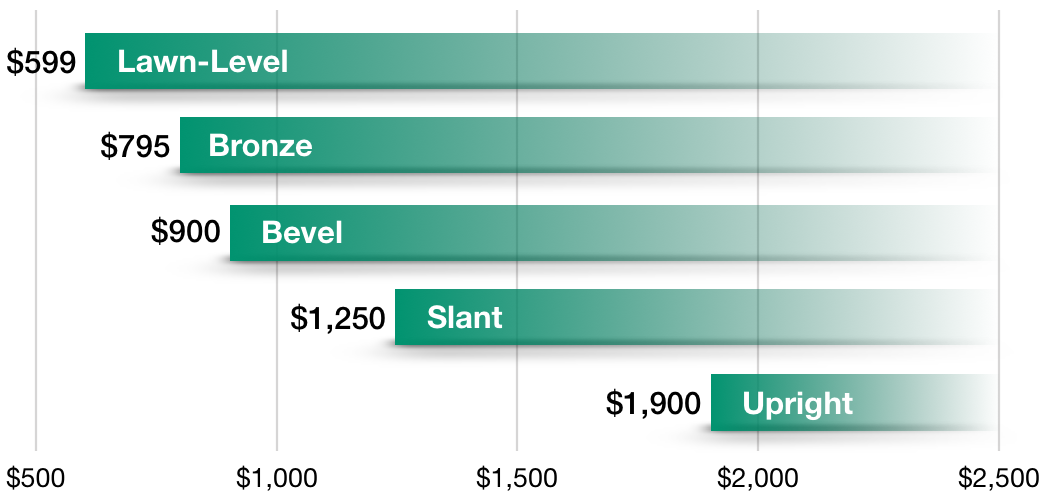
Critique the following graphic visualization of data: could it have been better represented in a different format? Is there anything misleading about the visualization?

Practice Quiz 1 Solutions
A pie chart or a bar chart. Since there are only two responses, each person can only select one answer, and the pie chart often gives a relatively clear sense of which proportion picked which answer. A bar chart could also work well, and humans are better at judging bar heights than angles.
A scatterplot; this allows us to visually see if there is an association between these two parameters.
A not-as-good (but reasonable in some circumstances) answer would be a pair of histograms (on different axes); this would give us a sense of how each individual variable (BMI and cholesterol) are distributed in the patient population.
When it is presented as a bar chart, it makes it seem like each bar is comparable to all of the other bars, but here they are in two categories, year + age. The data measures how a single measurement changes over time, and could be better presented as 4 separate time series, one for each age group. That would also make the data easier to compare.
Practice Quiz # 2#
The registrar reports that the average Stanford GPA is 3.45 for first-years, 3.51 for second-years, 3.58 for third-years, and 3.69 for fourth-years (in the interest of full disclosure, I actually made this data up). What kind of graphic would you use to visually summarize this data, and why?
A city monitors wastewater for infectious diseases. Suppose city officials take weekly measurements of the concentration of bird flu virus in the wastewater. What kind of graphic would you use to visually summarize this data, and why?
Critique the following graphic visualization of data: could it have been better represented in a different format? Is there anything misleading about the visualization?
Practice Quiz 2 Solutions
A bar chart, because we have a numerical quantity and we are comparing its value across a number of different categories.
A time series. We are tracking how a single measurement evolves over time.
This visualization is misleading because it is a bar chart where (a) the not-colored-in part of the bar actually represents how large the quantity is, and (b) even if the bars were properly colored in, the value for bars does not start at 0, and the right-hand-side is set to make the most expensive option look best.
Practice Quiz #3#
You survey 1000 people and you ask them for (a) their annual salary and (b) how many days of vacation they take per year. What kind of graphic would you use to visually summarize this data, and why?
An ecologist has taken measurements of the beak length of 1000 randomly captured birds (all of the same species). What kind of graphic would you use to visually summarize this data, and why?
Critique the following graphic visualization of data: could it have been better represented in a different format? Is there anything misleading about the visualization?

Practice Quiz 3 Solutions
A scatterplot; this allows us to visually see if there is an association between these two parameters.
A not-as-good (but reasonable in some circumstances) answer would be a pair of histograms (on different axes); this would give us a sense of how each individual variable (salary and vacation days) are distributed in the patient population.
A histogram, because this is a result of a numerical sample and we will get a sense of how beak length is distributed in the population.
The type of quantities plotted in this time series are all of the same category: military expenditure by various countries. Yet, the Y-axes differ on the left and right hand sides, and every country except the U.S. is plotted according to the left axis, whereas the US is plotted according to the right axis. Also the right axis does not start at zero. The U.S. line would actually start above the top of the chart if it were plotted according to the left axis.
Week 5: Fundamental summary statistics#
Practice Quiz #1#
For the dataset below, calculate the mean, median and standard deviation.
Section Attendance, week of April 21
TA |
Attendees |
|---|---|
Aditya |
15 |
Ginnie |
13 |
Ian |
15 |
Leda |
1 |
Michael |
8 |
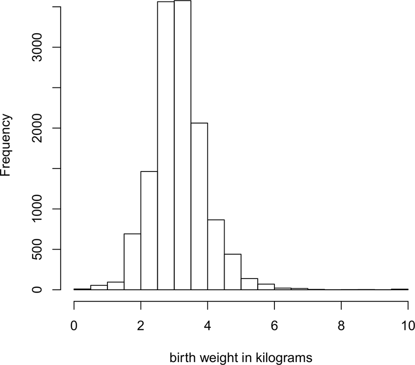
In the dataset represented by the top histogram below, is the mean a. About the same as the median, b. Larger than the median, or c. Smaller than the median?
Explain why you think your answer is correct. (Even if your answer is technically incorrect, you’ll get full credit if your reasoning is sound—we don’t expect you to compute the mean and median).
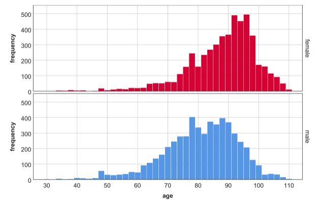
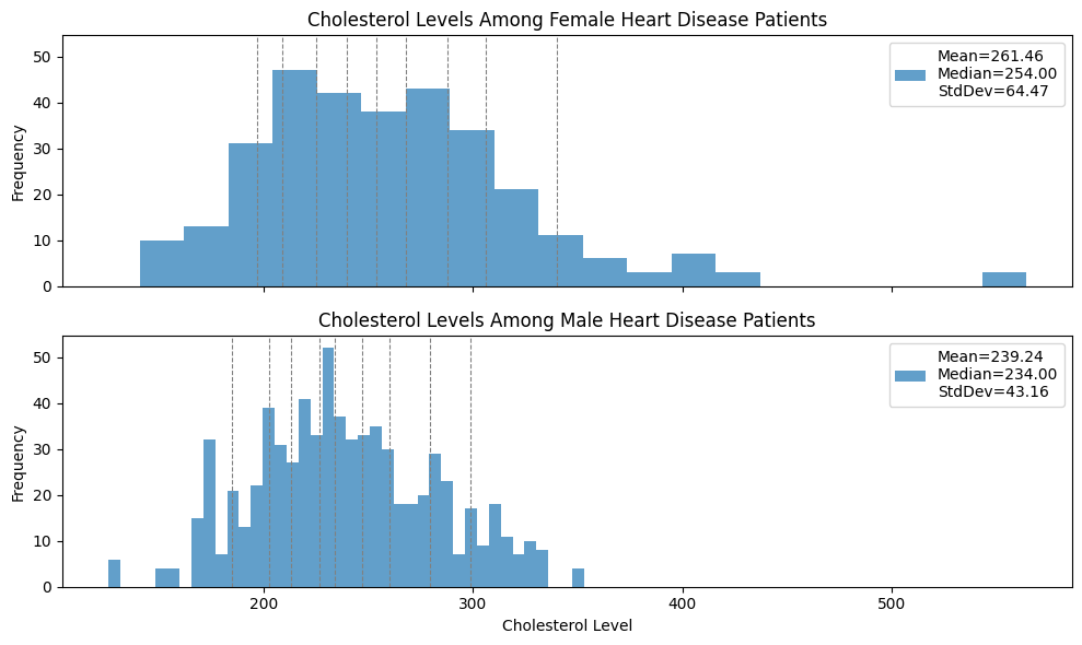
Which of the two distributions exhibits greater variability? Justify your answer with an appropriate quantitative measure of variability.
Practice Quiz 1 Solutions
The mean is \(\frac{1}{5}\left(15 + 13 + 15 + 1 + 8\right) = 10.4\)
The standard deviation is \(\sqrt{\frac{1}{5}\left((15-10.4)^2 + (13-10.4)^2 + (15-10.4)^2 + (1-10.4)^2 + (8-10.4)^2\right)} \approx 5.4\).
The median is 13.
It looks like the mean is smaller than the median; the distribution looks heavy-tailed on the left, with the highest frequencies on high numbers, and then many entries spread out over low numbers, which usually decreases the mean relative to the median.
The Cholesterol level among female patients exhibits higher variability. The means are pretty close and the standard deviation is a factor 2/3 larger, and also the distance between the 90th and 10th percentiles is larger.
Practice Quiz # 2#
For the dataset below, calculate the mean, median and standard deviation.
Points scored by LeBron James in 2017 NBA finals games
Game |
Points |
|---|---|
1 |
28 |
2 |
29 |
3 |
39 |
4 |
31 |
5 |
41 |
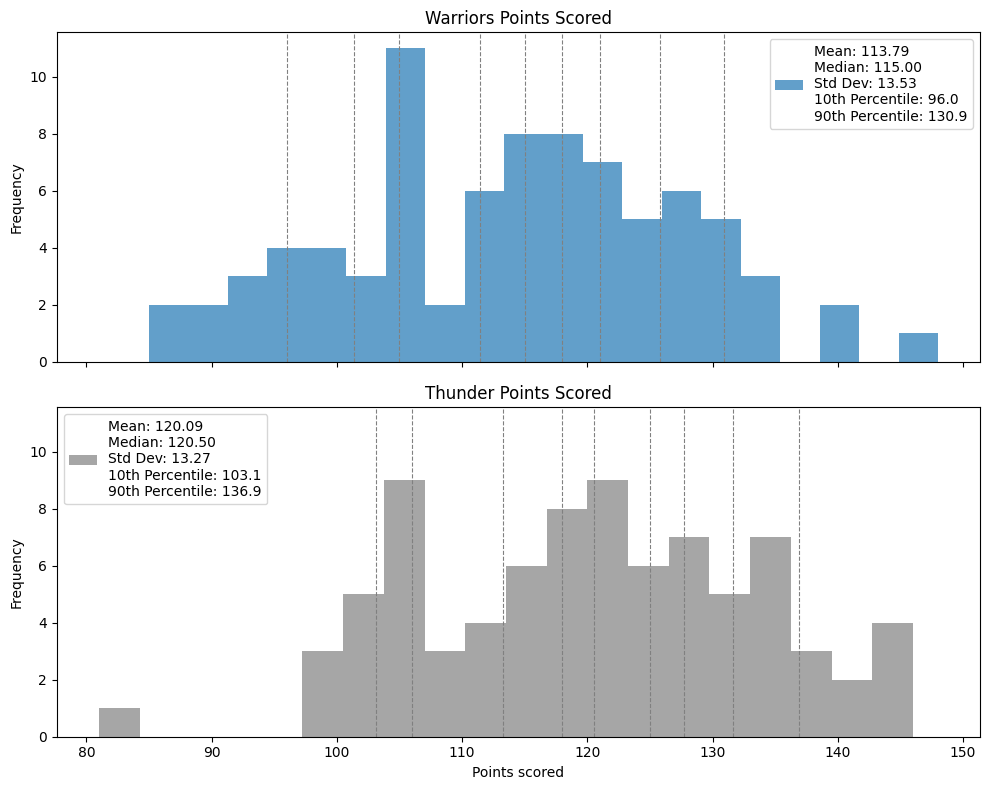
In the dataset represented by the histogram below, is the mean a. About the same as the median, b. Larger than the median, or c. Smaller than the median?
Explain why you think your answer is correct. (Even if your answer is technically incorrect, you’ll get full credit if your reasoning is sound—we don’t expect you to compute the mean and median).

Which of the two distributions exhibits greater variability? Justify your answer with an appropriate quantitative measure of variability.
Practice Quiz 2 Solutions
The mean is \(\frac{1}{5}\left(28 + 29 + 39 + 31 + 41 \right) = 33.6\).
The standard deviation is \(\sqrt{\frac{1}{5}\left((28-33.6)^2 + (29-33.6)^2 + (39-33.6)^2 + (31-33.6)^2 + (41-33.6)^2 \right)} \approx 5.4\).
The median is 31.
It looks like the mean is larger than the median; the distribution looks heavy-tailed on the right, with the highest frequencies on low numbers, and then many entries spread out over high numbers, which usually pulls up the mean relative to the median.
The Warriors points distribution exhibits greater variability; the distance between the median and 10th percentile is almost 30 points, whereas the thunders’ is less than 20. Also, there are more outliers, the distance between the 10th and 90th percentile is slightly larger, and the standard deviation is also slightly larger.
Practice Quiz #3#
For the dataset below, calculate the mean, median and standard deviation.
Max daily temperature in San Francisco
Date |
Max Temp (F) |
|---|---|
4/21/25 |
70 |
4/22/25 |
68 |
4/23/25 |
58 |
4/24/25 |
56 |
4/25/25 |
60 |
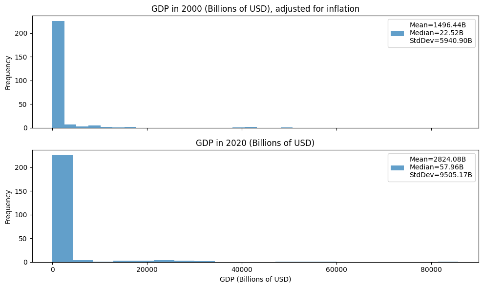
In the dataset represented by the histogram below, is the mean a. About the same as the median, b. Larger than the median, or c. Smaller than the median?
Explain why you think your answer is correct. (Even if your answer is technically incorrect, you’ll get full credit if your reasoning is sound—we don’t expect you to compute the mean and median).
Which of the two distributions exhibits greater variability? Justify your answer with an appropriate quantitative measure of variability.
Practice Quiz 3 Solutions
The mean is \(\frac{1}{5}(70+68+58+56+60) = 62.4\).
The Standard deviation is \(\sqrt{\frac{1}{5}\left((70-62.4)^2 + (68-62.4)^2 + (58-62.4)^2 + (56-62.4)^2 + (60-62.4)^2)\right)} \approx 5.5\).
The median is \(60\).
The mean and median look about the same; the histogram looks like it is roughly balanced around the center.
The variability of the 2020 data is higher. The standard deviation is almost twice as large. The gap between the mean and median is also almost twice as large, which reflects the presence of more outliers.
Week 6: Estimating from a sample#
Practice Quiz #1#
Decide whether the following statement is True or False, and justify your answer:
“The Normal Approximation of the sample mean applies, no matter how the samples are collected”
In the following scenario, explain
a. What is the population
b. What is the variable \(x\) being measured
c. What is the sample \(x_1,\ldots,x_n\)
An economist wants to estimate what percent of the average San Francisco restaurant servers’ earned income comes from tips. The economist looks at the municipal tax records, picks 100 random people who list their occupation as “restaurant server”, and calls them to ask them what percent of their earned income last year was from tips.
You are trying to estimate the proportion of left-handed people on Stanford campus (about 10% of people in the population overall are left-handed). Suppose you survey \(n = 50\) students and compute the proportion who were left-handed, \(\hat\mu_n\). Can you be \(68\%\) confident that \(|\hat\mu_n - \mu| \le \frac{\sigma }{\sqrt{n}}\)?
Practice Quiz 1 Solutions
False. It is important that the data points are collected independently and uniformly.
In this scenario, the population is the San Francisco restaurant servers, and the variable \(x\) is the percent of the server’s income that came from tips last year. The sample is, for each contacted server, the percent \(x_i\) that this specific server made from tips in the last year.
No. The Normal approximation does not apply since we expect to have \(p \approx \frac{1}{10}\) and so \(\min(np,n(1-p)) \approx 5 < 10\).
Practice Quiz 2#
Decide whether the following statement is True or False, and justify your answer:
“A larger sample size makes confidence intervals for the sample mean smaller while also increasing confidence.”
In the following scenario, explain
a. What is the population
b. What is the variable \(x\) being measured
c. What is the sample \(x_1,\ldots,x_n\)
A penguin ecologist is trying to determine the average number of offspring a female Antarctic penguin will hatch over her lifetime. The ecologist tags \(n\) Antarctic female penguins at random, then returns to Antarctica each year over a period of 20 years to observe whether the tagged penguins succeed in hatching their eggs.
Suppose you conduct a poll on an issue on which the population is roughly divided (you expect about half the people will answer yes). You survey \(n=25\) people and compute the proportion who said yes, \(\hat\mu_n\). Can you be \(95\%\) confident that \(|\hat\mu_n - \mu| \le 2 \frac{1}{\sqrt{n}}\)?
Practice Quiz 2 Solutions
True.
Increasing \(n\) decreases the standard deviation of the sample mean, which makes us both more confident that \(|\hat\mu_n - \mu| \le \epsilon\) for a fixed \(\epsilon\), and also \(95\%\) confident that \(|\hat\mu_n - \mu| \le 2\frac{\sigma}{\sqrt{n}}\), a window that shrinks with \(n\).
In this scenario, the population is the Antarctic female penguins, and the variable \(x\) is the number of eggs that a female hatches over the course of her lifetime. The sample is, for each tagged female penguin, the number of eggs \(x_i\) that the female hatched over the 20 year period that the ecologist observed her.
Yes. The Normal approximation applies since we have \(p \approx \frac{1}{2}\) and so \(\min(np,n(1-p)) \approx 12 > 10\). Since this is a poll, we can take \(1\) as an upper bound on \(\sigma\). Then, the 68-95-99 rule implies that there is a 95% chance that \(\hat\mu_n\) is within 2 standard deviations of \(\mu\).
Practice Quiz #3#
Decide whether the following statement is True or False, and justify your answer:
“The Normal Approximation of the sample mean applies, no matter how small the sample size is”
In the following scenario, explain
a. What is the population
b. What is the variable \(x\) being measured
c. What is the sample \(x_1,\ldots,x_n\)
An engineer has designed a new machine for injecting medication for heart attack victims. It is important that the injection is deployed as quickly as possible. In order to determine the mean deployment time, the engineer tests out the machine on artificial tissue in the lab \(n\) times.
Suppose you conduct a yes/no poll on a controversial issue, where approximately half of the population likely answer “yes”. If you survey \(100\) people and let \(\hat\mu_n\) be the proportion of those surveyed who answered “yes”, can you be 68% confident that \(\hat\mu_n\) is within \(\frac{1}{10}\) of the fraction of people in the population who would answer “yes”?
Practice Quiz 3 Solutions
False. If \(n\) is too small, say \(n=1\), then the distribution of \(\hat \mu_n\) is the same as the population distribution which does not need to be normal. It could e.g. be the distribution of the outcome of a coinflip.
In this scenario, the “population” is the uses of the machine. The variable \(x\) is the amount of time it takes to deploy the injection. The sample is \(n\) different trials of the machine, and each \(x_i\) is the amount of time it took to deploy the medication on the \(i\)th trial.
Yes; the poll is like a coinflip with heads probability \(p \approx \frac{1}{2}\), and we do \(n=100\) trials \(\min(np,n(1-p)) \approx 50 > 10\), so the normal approximation applies. We are within one standard deviation with confidence \(68\%\), and here a standard deviation for the sample mean is \(\sigma/\sqrt{100} = \sigma/10 \le \frac{1}{10}\).
Week 7: Hypothesis Testing#
Practice Quiz #1#
You are a penguin ecologist in Antarctica.
You arrive at a new Antarctic island, where you sample \(n=100\) penguins and determine that the sample mean body mass of penguins on this island is \(3\) kilograms.
The population mean penguin weight for other Antarctic islands is \(4\) kilograms, and the population standard deviation is \(0.5\) kilograms.
Based on the data you collected, the penguins on this new island seem generally slimmer.
Formulate a hypothesis test to decide if the phenomenon described is a statistically significant pattern, or is likely to be random noise. You may assume your sample size is large enough so that the Normal Approximation for the sample mean applies.
What is the null hypothesis?
What is the \(p\)-value?
Decide whether you should reject the null hypothesis, and state the false positive (type 1 error) rate for your test.
Practice Quiz 1 Solutions
The sample size is \(n=100\), sample mean is \(\hat\mu=3\) and the population s.d. is \(\sigma=0.5\).
Let \(\mu\) be the population mean body mass of penguins on this island. The null hypothesis is that the mean body mass on the island is no different from elsewhere in Antarctica, \(H_0:\mu=4\). (Optional: we test \(H_0:\mu=4\) against the alternative \(H_1:\mu<4\)).
We observed the sample mean, \(\hat\mu = 3\).
Under the null hypothesis, the magnitude of the difference between the sample mean and the population mean is \(|\hat\mu - \mu| = |3-4| = 1\).
Taking the Normal approximation, the standard deviation of \(\hat\mu_n\) is \(\frac{.5}{\sqrt{n}} = \frac{.5}{\sqrt{100}} = \frac{1}{20}\), and the outcome we observed was \(\frac{1}{\frac{1}{20}} = 20\) standard deviations away from \(\mu\).
Applying the 68-95-99 rule, the probability that \(\hat\mu_n\) is \(20\) standard deviations away from the mean, under the normal approximation, is much less than \(1\%\).
So the \(p\)-value is \(< 0.01\).
Since \(p\ll 0.05\), we reject the null hypothesis (which supports the statement that the penguins on this new island seem generally slimmer). The false positive (or type I error) rate is \(\alpha = 0.05\).
Practice Quiz # 2#
A Stanford professor is teaching Calculus. For the first time, she decides to eliminate homework, and she wants to measure the impact this has on final exam performance.
In previous years, half of students get \(85\%\) or better on the final exam.
This year, in a class of size \(n = 100\), 45 students got \(85\%\) or better on the final exam.
Formulate a hypothesis test to decide if the phenomenon described is a statistically significant pattern, or is likely to be random noise.
What is the null hypothesis?
What is the \(p\)-value? You may use the Normal Approximation.
Decide whether you should reject the null hypothesis, and state the false positive (type 1 error) rate for your test.
Practice Quiz 2 Solutions
The sample size is \(n=100\). Let \(p_0\) be the chance that a student gets \(\ge 85\%\) on the final exam.
The null hypothesis is that the students mastered the material just as well as in previous years, and that \(p_0 = 0.5\).
We can probabilistically model the final hypothesis as: each student gets \(85\%\) or better independently with probability \(p_0 = 0.5\).
Under the null hypothesis, the chance that \(45\) or fewer students get 85% on the final exam is
Since \(n p_0\) and \(n(1-p_0)\) are both at least 10, we can take the normal approximation to get an approximate \(p\)-value.
We have \(\hat p = \frac{45}{100}\) the sample mean, an upper bound of \(\frac{1}{2\sqrt{100}} = 1/20\) on the standard deviation of the sample mean.
The distance from \(\hat p\) to \(p_0\) is \(0.05\), which is \(1\) standard deviation.
So using the 68-95-99 rule, the \(p\)-value is \(1-.68 = .32\).
Note: we would also accept a one-sided \(p\)-value, which computes the probability that \(\hat p - p_0 \le -.05\); this would have given a \(p\)-value of \(0.16\).
Since the p-value is more than 0.05, we fail to reject the null hypothesis \(H_0\). The false positive (or type I error) rate is \(\alpha = 0.05\).
Practice Quiz #3#
A candy company promises that at least \(50\%\) of their chocolate eggs contain a figurine of the fictional character Elsa from Frozen; the rest contain other toys. Suppose you buy \(n = 100\) chocolate eggs at random, and only \(40\) of them contain an Elsa figurine.
You suspect that the company is lying about the proportion of Elsas.
Formulate a hypothesis test to decide if the phenomenon described is a statistically significant pattern, or is likely to be random noise.
What is the null hypothesis?
What is the \(p\)-value?
Decide whether you should reject the null hypothesis, and state the false positive (type 1 error) rate for your test.
Practice Quiz 3 Solutions
The sample size is \(n=100\). Let \(p_0\) be the population proportion of chocolate eggs containing a figurine of the fictional character Elsa from Frozen. We observed \(\hat{p}_0=40/100=0.4\).
The null hypothesis is that the company is telling the truth about the proportion of Elsa eggs, \(H_0: p_0=0.5\). (Optional: we will test \(H_0: p_0=0.5\) against the alternative \(H_1:p_0<0.5\)).
We observed \(|\hat p - p_0| = 0.1\). Taking the Normal approximation for \(\hat p\), we have that its standard deviation is at most \(\frac{0.5}{\sqrt{n}} = \frac{1}{20}\). The difference \(|\hat p - p_0| = 0.1\), which is two standard deviations.
Taking the normal approximation for \(\hat p\) and applying the 68-95-99 rule, the probability that \(|\hat p - p_0| \ge 0.1\) is at most \(1-.95 = 0.05\).
Since the p-value is less than 0.05, we reject the null hypothesis \(H_0\). The false positive (or type I error) rate is \(\alpha = 0.05\).
Week 8: Experimental Design#
Practice Quiz #1#
In each of the following experiments (a) list the strengths and weaknesses of each experimental design, (b) state whether you think the experiment will be effective at answering the experimenters’ question, and if not, suggest an alternative design that would be more effective.
An elementary school wants to decide between two choices of curriculum for teaching reading: A or B. The school has 100 pupils in each grade, each divided into 4 equal classrooms of size 25. The administration decides to run the following experiment: they will randomly assign two kindergarten classes to curriculum A, and the remaining two to curriculum B, and at the end of a 1 year period they will give each student a reading assessment, and use the results to determine if A or B was better.
A marketer wants to determine whether people are more likely to buy product A or product B. They do a survey, choosing 100 random customers and asking each one of them if they are more likely to buy A or B.
A psychiatrist is trying to determine whether there is a causal relationship between sleep and positive social interactions. The psychiatrist surveys 1000 people, asking each (1) how many hours of sleep they get on a typical night, and (2) how positive are their social interactions on a scale from 1-10. The psychiatrist then measures the correlation coefficient of these variables.
Practice Quiz 1 Solutions
Relatively effective.
Strengths: Randomization at the classroom level helps control for confounding variables at that level (e.g., classroom assignment isn’t based on ability). Same assessment is used for all students, ensuring consistent measurement.
Weaknesses: If each classroom has a different teacher, the effect of curriculum is confounded with teacher quality or teaching style. The study is limited to kindergarten so if the school wants to apply this across all grades, results may not extrapolate. With only 2 classrooms per treatment, there could be too much noise from teacher quality to make a conclusion about the choice of curriculum.
Proposed changes to make more effective: randomize more classrooms per treatment, potentially across multiple grades or schools. Rotate teachers across treatments to remove teacher quality confounding.
Not very effective.
Strengths: Random sample of customers.
Weaknesses: Stated preferences can differ from actual behavior. There is no random assignment and no control for confounding variables (eg. demographics, purchase history, etc.)
Proposed changes to make more effective: make this a truly randomized experiment by randomly showing a customer either A or B in a purchase setting, and measuring real purchase rates.
Not very effective.
Strengths: Large sample size
Weaknesses: Survey response bias, people can misreport their hours of sleep, no standardized way of measuring amount of sleep, social interactions are rated on a subjective scale, and no consideration for confounding variables (eg. mental health, job stress, age, etc.) No random assignment.
Proposed changes to make more effective: make this a truly randomized experiment by assigning participants to a sleep intervention group versus a control group, and measuring outcomes over time
Practice Quiz # 2#
In each of the following experiments (a) list the strengths and weaknesses of each experimental design, (b) state whether you think the experiment will be effective at answering the experimenters’ question, and if not, suggest an alternative design that would be more effective.
An election forecaster wants to predict whether it is more likely that candidate A or candidate B will win a county election. The race is expected to be close; the voting population of the county is \(100,000\), and both of the previous elections were decided by about \(500\) votes. The forecaster carefully chooses a uniform sample of 100 voters in the county, and asks them who they plan to vote for.
A behavioral economist wants to determine whether people are more likely to perform tasks voluntarily when they are in a good mood. The economist runs a randomized control trial on students in their ECON 101 class, assigning half of them randomly to a treatment group and half to a control group. Students in the control group are asked if they are willing to help clean a chalkboard. Students in the treatment group are first told that they scored well on an exam, then asked if they are willing to help clean a chalkboard.
A politician wants to determine which stump speech is more effective to give on the campaign trail. In order to decide, he gives version A of the speech at the first stop on the trail, and version B at the second stop, and then goes with the version that received a more enthusiastic response.
Practice Quiz 2 Solutions
Not very effective.
Strengths: Random sample of constituents
Weaknesses: Sample size is too small so the margin of error is too high for this tight race (with high confidence the sample mean error for a proportion is on the order of \(1/\sqrt{n}\), and we need an error less than \(500/100000\), so we require a sample size of \(n\) on the order of \(10,000\)). There is survey response bias and the race is constantly evolving so responses obtained by the survey may change between now and the election.
Proposed changes to make more effective: ideally collect a much larger sample size to mitigate some of the issue raised in the weaknesses section.
Effective.
Strengths: Random treatment assignment, being told of good exam score is a straightforward way to induce a good mood, willingness to help clean whiteboard is easy response to measure.
Weaknesses, proposed changes: none of note.
Not very effective.
Weaknesses: The treatment is not randomly assigned, the demographics of the audience at each stop can be totally different and delivery of the speech may differ from stop to stop. Due to crowded behavior, positive or negative reception of the speech can be amplified.
Proposed changes to make more effective: Make this a randomized experiment by randomly assigning speech versions across many similar audiences and measuring outcomes consistently (e.g., applause duration, follow-up engagement).
Practice Quiz #3#
In each of the following experiments (a) list the strengths and weaknesses of each experimental design, (b) state whether you think the experiment will be effective at answering the experimenters’ question, and if not, suggest an alternative design that would be more effective.
A team of medical researchers is trying to determine which dosage of blood thinner is most effective at preventing strokes in heart disease patients. They run a randomized trial across ten hospitals in ten large US cities. Within each hospital, every patient is assigned randomly in a double-blind manner to either dose A or dose B, and the number of strokes in each group is tracked over a 5 year period.
A city is trying to determine what the best strategy is for decreasing auto break-ins. The city council decides to increase police patrols in the problematic areas and see if the number of break-ins decreases.
A health advocate is trying to determine whether caffeine consumption causes negative mental health outcomes. The advocate conducts a survey of \(10,000\) randomly chosen U.S. adults, and asks each of them about (1) their caffeine consumption habits and (2) their mental health.
Practice Quiz 3 Solutions
Effective
Strengths: Randomization within hospitals, double blind design prevents biases, study performed across 10 large hospitals increases robustness, long followup period of 5 years.
Weaknesses: Does not account for confounding variables in the respective patient populations, patients can drop out of study in 5 years
Proposed changes to make more effective: within-hospital randomization done separately per hospital to control for potential systematic differences in patient demographics.
Not very effective.
Weaknesses: No randomized treatment, there is no clear measurement, no way to address confounding variables.
Proposed changes to make more effective: Create a randomized treatment by assigning (randomly) some high crime areas to increased patrol and others to the status quo.
Not very effective.
Weaknesses: Adults are randomly selected to answer survey but this has nothing to do with randomly assigning a treatment. There is no mention of confounding variables (eg. stress, work habits, lifestyle, etc.) There is self-reporting bias in survey results. Cannot establish causal relationship from observational study.
Proposed changes to make more effective: Randomize treatment by assigning people to reduce caffeine intake (and others to have a specified non-reduced amount of caffeine).