Lecture 26: Nearest Neighbors#
STATS 60 / STATS 160 / PSYCH 10
Concepts and Learning Goals:
The \(k\)-nearest neighbors model
Classification
Effects of selection bias in training data
Return to admissions#
Imagine you work in the admissions office.
You want to use applicants’ SAT percentiles \(x_{SAT}\) to predict \(y\), their freshman year GPA if they were to be admitted.
Last time, we trained a linear regression model \(f\) to generate a prediction \(\hat{y}\),
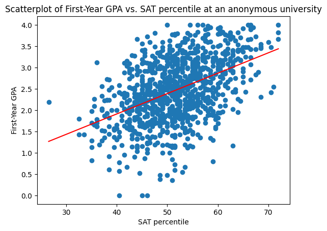
Today, we’ll see a different model: the \(k\)-Nearest-Neighbors model.
Compatible?#
Your high school friend has just moved to the bay area. Your roommate wants you to set them up on a date.
Question: How do you decide if they will be compatible?
One common strategy is comparison:
How similar is your roommate to your friends’ past relationships?
Were those relationships good or bad?
\(k\)-Nearest-Neighbors#
Assume we have access to a set of examples of features \(x\) and labels \(y\),
We are given a new datapoint \(x\), and we want to generate a prediction \(\hat y\) for \(y\).
The \(k\)-Nearest Neighbors Model:
Find the \(k\) examples \(x_{i_1},x_{i_2},\ldots,x_{i_k}\) most similar to \(x\).
In case of a tie in similarity, increase \(k\) to include all the tied points.
Choose our prediction \(\hat{y}\) to be the average of \(y_{i_1},\ldots,y_{i_k}\).
Nearest Neighbor Prediction#
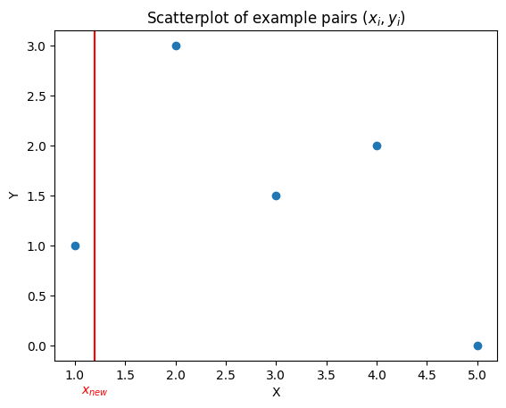
Question: what would your \(1\)-nearest-neighbor prediction for the point \(x_{new}\) be?
Question: what would your \(2\)-nearest-neighbor prediction for the point \(x_{new}\) be?
\(k\)-Nearest-Neighbors for first-year GPA#
Below are the prediction curves for the first-year GPA produced by \(k\)-Nearest-Neighbors for \(k = 1,5,10,20,30\).
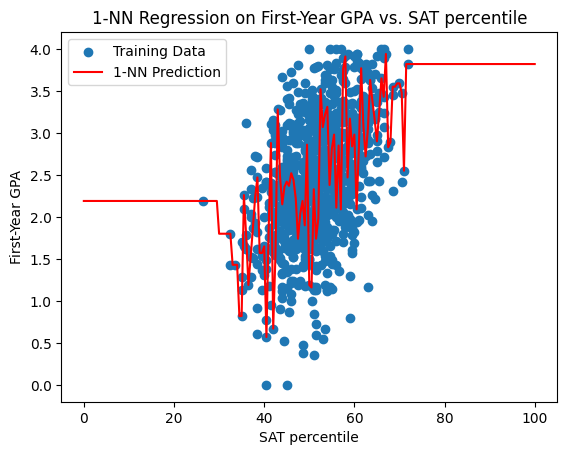
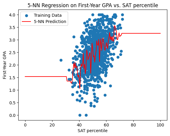
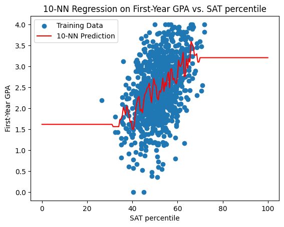

What happens as we vary \(k\)?#
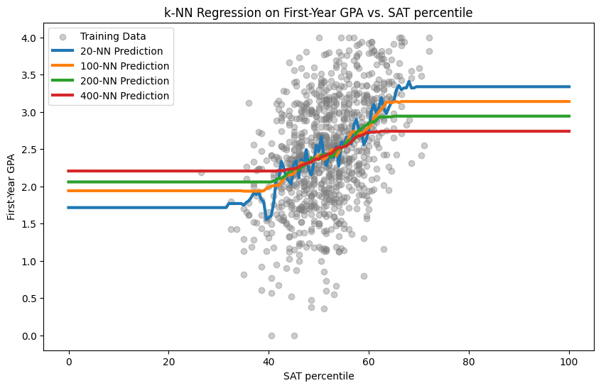
Question: what do you notice about the \(k\)-nearest neighbor model prediction as \(k\) increases?
Question: do you see a disadvantage to taking \(k\) too small?
Question: do you see a disadvantage to taking \(k\) too large?
Evaluating the model#
To evaluate the \(k\)-nearest-neighbors model for regression, we’ll use root mean squared error (just like for linear regression).
Question: Assume that we only have one example data point with features \(x_i\).
If \(k = 1\), what will \(\hat y = f(x_i)\) be?
Within the set of examples, \(x_i\) will be its own nearest neighbor, and the \(\hat y = y_i\).
So when \(x_i\) are all distinct, the model has zero error on our example data.
When \(x_i\) are not distinct, \(\hat y\) is still possibly very influenced by \(y_i\).
Because of this, the root mean squared error on our training examples is not a good measurement of accuracy.
Training data vs. Testing data#
To avoid cheating on our error measurement, in advance, we randomly split our example data into two parts: training data and testing data.
We train/define the model using the training data.
We evaluate model performance on the testing data.
It is actually a good idea to do this training/testing split even when we are evaluating a linear model.
But it is not as essential in the case of linear regression when the number of examples is big and when the influence of outliers is small.
Error for \(k\)-nearest neighbors#
For our \(k\)-nearest neighbor model for first-year GPA, the root mean squared error on the test data was:
\(k\) |
RMSE |
|---|---|
1 |
0.94 |
5 |
0.74 |
10 |
0.70 |
20 |
0.68 |
200 |
0.69 |
400 |
0.71 |
The value for \(k=20\) compares favorably with RMSE \(0.66\) for the best-fit linear model.
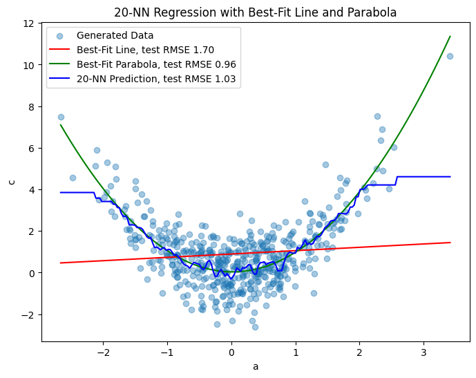
\(k\)-nearest neighbors and nonlinear data#
\(k\)-Nearest Neighbors can capture nonlinear relationships between \(x,y\).
Consider the synthetic quadratically associated data from Lecture 25:
Linear regression vs. \(k\)-nearest neigbhors#
Question: brainstorm as many advantages and disadvantages as you can for using \(k\)-nearest neighbors vs. linear regression.
Nonlinear associations: nearest neighbors is better
Interpretability: nearest neighbors arguably easier to understand
Effect of selection bias and outliers: it depends
Model selection: linear regression has a formula. Requires us to make fewer choices (no need to choose \(k\))
Classification#
In the examples we saw so far, the quantity \(y\) was a number. When you want to predict a number, that’s called a regression problem.
In classification problems, \(y\) takes a yes/no value, or a categorical value.
Examples:
Admissions: you want to predict whether or not a student passes freshman year.
Medicine: \(x\) is test results for a patient, and \(y\) is whether or not they have a disease.
Weather: \(x\) is temperature/pressure/humidity data, \(y\) is whether or not it is going to rain.
\(k\)-Nearest Neighbors for classification#
Assume we have access to a set of examples of features \(x\) and labels \(y\) (taking yes/no values),
We are given a new datapoint \(x\), and we want to generate a yes/no prediction \(\hat y\) for \(y\).
\(k\)-Nearest Neighbors:
Find the \(k\) examples \(x_{i_1},x_{i_2},\ldots,x_{i_k}\) most similar to \(x\)
Choose our prediction \(\hat{y}\) to be the majority of \(y_{i_1},\ldots,y_{i_k}\).
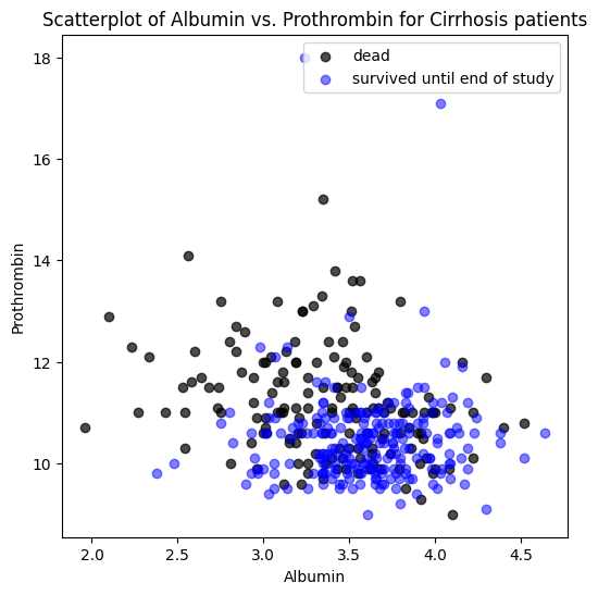
Example 1: Cirrhosis#
Cirrhosis is a chronic liver disease. This data comes from a study at the Mayo Clinic which ran from 1974 to 1984.
Below we have plotted patient measurements of two liver proteins, Albumin and Prothrombin, color coded according to whether they survived until the end of the study.
Decision Boundary#
We train a \(k\)-NN model to predict whether a patient with features \((x_{A},x_P)\) will survive.
k=1
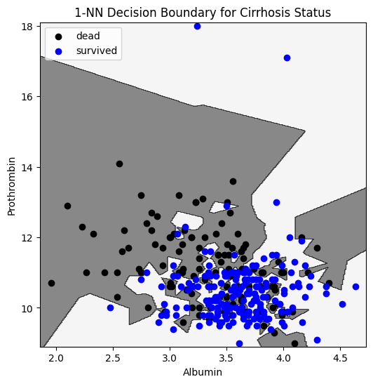
Evaluation on test set:
\(56\%\) of deaths classified as deaths
\(57\%\) of survivals classified as survivals
We can plot the decision boundary: our model predicts that a patient with measurements \((x_A,x_P)\) in the white region will survive.
k=10
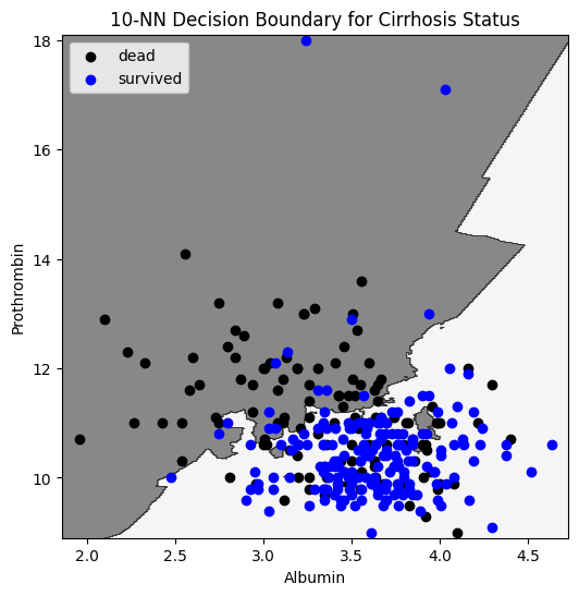
Evaluation on test set:
\(63\%\) of deaths classified as deaths
\(89\%\) of survivals classified as survivals
k=20
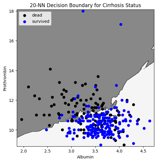
Evaluation on test set:
\(50\%\) of deaths classified as deaths
\(85\%\) of survivals classified as survivals
Example 2: Breast Cancer#
The following data describes features of tumors, along with a diagnosis of malignant or benign.
Below we have plotted measurements of two features of the tumor: concave points and texture.
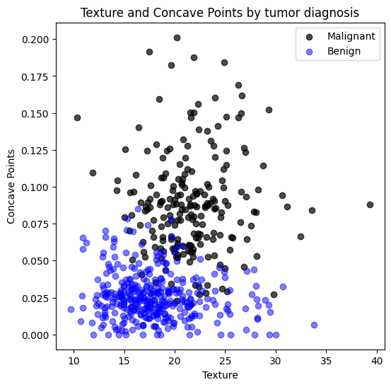
#
We train a \(k\)-NN classifier, and plot the decision boundary:
k=1
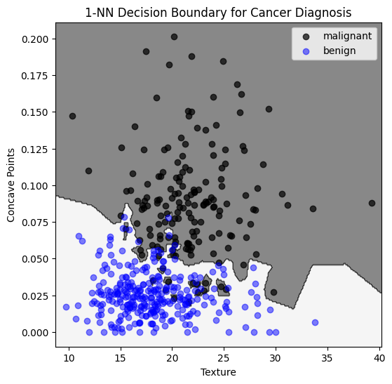
Evaluation on test set:
\(92\%\) of benign classified as benign
\(81\%\) of malignant classified as malignant
k=5
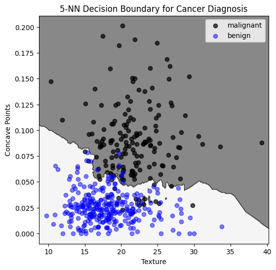
Evaluation on test set:
\(94\%\) of benign classified as benign
\(93\%\) of malignant classified as malignant
k = 20
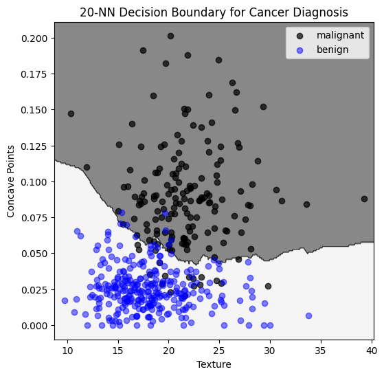
Evaluation on test set:
\(94\%\) of benign classified as benign
\(94\%\) of malignant classified as malignant
Regions with low coverage#
Question: Can we trust a diagnosis from the model on features \(x\) if \(x\) happens to fall in the bottom right of this plot? Why or why not?
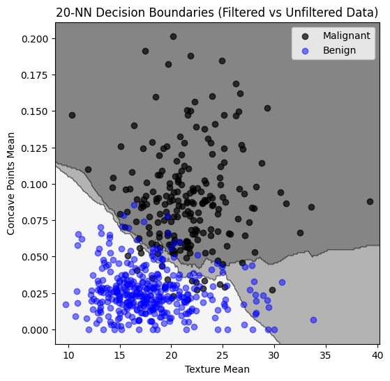
Selection bias#
The following \(20\)-NN model was trained on a training set that only included tumors on the larger side.
Only \(86\%\) of benign are classified as benign, compared to \(94\%\) with an unbiased training set.
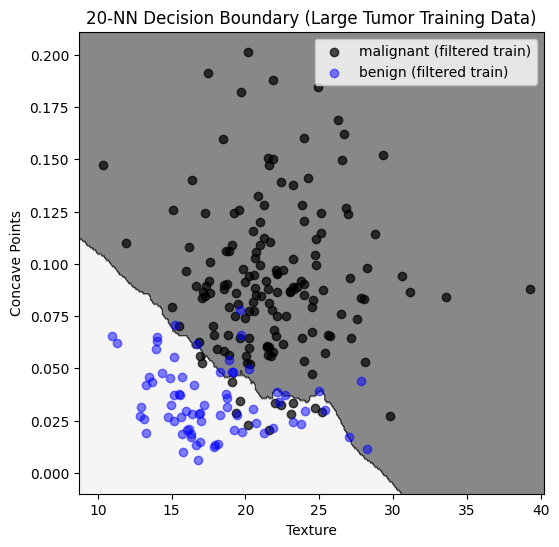
Here we have overlayed decision regions for the biased and non-biased sample. The biased training set causes more tumors to be classified as malignant.
Recap#
\(k\)-nearest neighbors model
Classification
decision boundary
Effect of selection bias in training set