Lecture 25: Intro to machine learning#
STATS 60 / STATS 160 / PSYCH 10
Announcements:
No quiz on Friday (due to short week)
Discussion tomorrow will be a review session. Bring your questions!
Practice final will be released next week.
Concepts and Learning Goals:
Prediction and models
Linear models and linear regression
Effect of training examples: sample size and selection bias
Decisions and Predictions#
Suppose you work in the admissions office. More than 40,000 students apply for about 2,000 slots each year.
You want to admit students who can succeed at Stanford; one metric of success is a good GPA at the end of freshman year.
For each applicant, you know their SAT percentile \(x_{SAT}\).
You want to use \(x\) to predict their Stanford freshman year GPA \(y\).
Models#
A model is a way to take in observed data \(x\) and output a decision or a prediction \(f(x) =\hat{y}\) for \(y\):
Here \(f\) is our model.
In the admissions scenario, our data is the applicant SAT percentile, \(x_{SAT}\), and we would like to predict \(y\), the applicant’s freshman GPA if they were to be admitted to stanford.
Now the goal is to come up with a model \(f\) which produces an estimate of \(y\), $\(\hat{y} = f(x_{SAT}).\)$
It is usually impossible to predict \(y\) exactly, because \(y\) depends on all kinds of unknown factors.
Our goal is to make the prediction error \(|\hat{y} - y|\) as small as possible.
First contact#
Let’s do an exercise:
Pair up with a teammate
One of you is an earthling, the other is an alien
The earthling should try to explain to the alien what the word “bitter” (as in the flavor) means
The alien should interact like they have genuinely never heard of this word before
Question: what kind of explanations were easiest to come up with? What kind of explanations were easiest to learn from?
Usually, it is easier to explain and learn through examples.
Training a model with data#
The modern approach in statistics and machine learning is to “train” a model \(f\) using examples.
Decide what type of model \(f\) to use.
For example, we might choose to make \(f\) a linear function of its input \(x\).
There are many other types of models; as the unit progresses we will see aother examples.
There are lots of possible linear functions. If the input \(x\) is a 1-dimensional variable, to determine \(f\) we need to choose a slope \(m\) and intercept \(b\): $\(f(x) = m \cdot x + b,\)$ The slope and intercept are the parameters or weights of the model.
Collect examples of pairs \((x_1,y_1),\ldots,(x_n,y_n)\); \(x_i\) are data, and \(y_i\) are the corresponding “correct” decisions.
Choose model parameters by training \(f\) on the example data.
“Training” means, select the parameters (slope, intercept) that fit our example data best.
The notion of “best fit” is up to us.
SAT vs. first-year GPA data#
Below is an anonymized dataset of 1000 example pairs \((x_{SAT},y)\) (from an unspecified college, not Stanford).

Now, we observe only the SAT percentile score \(x_{SAT}\) for a new applicant, and we want to produce a prediction \(\hat{y}\) of their first-year GPA, \(y\).
Linear Regression#
A simple example of a model is linear regression. If \(x\) is one-dimensional:
To specify \(f\), it is enough to choose values for the parameters \(m,b\).
How do we train \(f\) (that is, how do we choose the parameters)?
A simple and effective approach is to choose the parameters which minimize the mean squared error of \(f\) on our examples:
Linear regression for freshman GPA#
In the first-year GPA dataset, this is the best-fit line (computed using colab, which uses a formula):
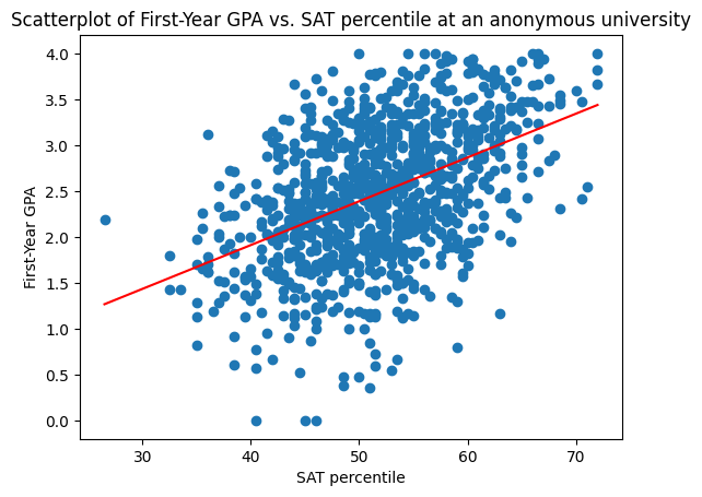
If the applicant scored in the \(83\)rd percentile, then \(x_{SAT} = 83\), and we predict
Error for freshman GPA#
Even for the examples that we used to train our model, there is some error.
For many examples \((x_i,y_i)\), \(|f(x_i) - y_i| > 0\)
Equivalently, many points do not lie on the line.
The root mean squared error for our model is $\( RMSE(f) = \sqrt{\frac{1}{n} \sum_{i=1}^n (f(x_i) - y_i)^2}.\)$
It measures how small the squared error is for our average example; the square root is taken so that we get the correct units.
In our SAT example, $\( RMSE(f) = 0.66 \text{ grade points}. \)$
Improving error with more features#
Using just the SAT percentile might not give very good predictions.
We can improve the error of our model by incorporating more features of each applicant: for example, we can incorporate high school GPA.
Our examples are now triples \((x_{SAT}, x_{GPA}, y)\):
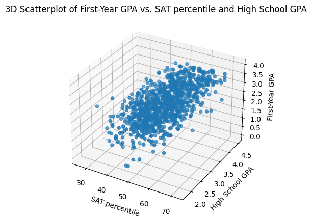
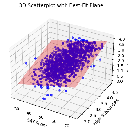
We can now fit a linear regression model with both variables, \(x_{SAT}\) and \(x_{GPA}\):
The interpretation is that we are trying to find a plane or flat surface, described by the parameters or weights \(m_1,m_2,b\) that has the minimum mean squared distance to our examples.
One advantage of linear models is that there is a formula for the best parameters. That isn’t true in every models; for example, it’s not true for deep networks.
Our root mean squared error has now improved:
Compare with \(0.66\) grade points, when we were using only \(x_{SAT}\).
Sample size and selection bias#
Think back to your human-alien interaction.
Question: How many examples do you think you would need before the alien really understands the definition of “bitter” well?
Question: What would happen if the examples you chose were biased? For instance, suppose your examples were all bitter liquids.
Just like when we try to estimate other quantities, prediction models tend to improve when you increase the number of examples and try to avoid selection bias.
Too few examples#
Let’s see what happens if we try to learn a model \(f\) using only 5 examples, instead of 1000:
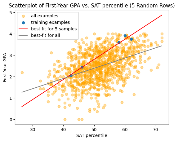
The model we learned tends to over-estimate the first-year GPA, and the root mean squared error on the whole dataset is larger,
compared with \(0.66\) grade points.
This is another example where adding more examples/samples decreases the variability of our estimate.
Selection bias#
Selection bias can impact the error or our model.
Here is a linear model \(f(x_{SAT})\) trained using only examples from students with high school GPA less than 3.0:
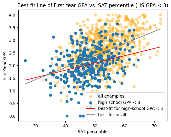
We can see that the line tends to under-estimate the first-year GPA for students with higher high-school GPAs.
The root mean squared error on all of the examples is
This is larger than the value \(0.66\) that we got on the whole dataset.
Limitations of the model#
The type of model also influences how good our prediction is.
For example, linear regression is a very bad model when \(y\) is quadratic in \(x\):
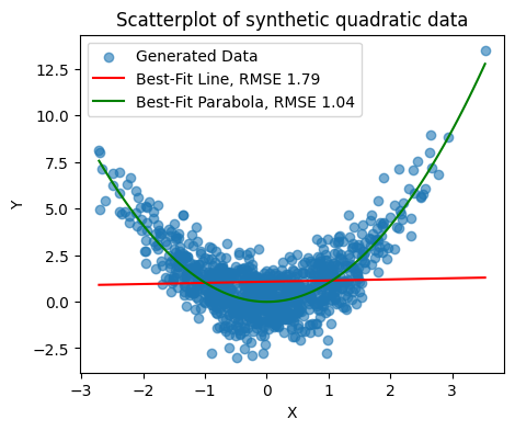
More on this in the next couple of lectures.
Recap#
Prediction and models
training from examples
Linear models and linear regression
Prediction error
root mean squared error
Improving performance:
Using more features of input
Larger sample size
Effect of selection bias