Lecture 8: Common mistakes in conditional logic

Lecture 8: Common mistakes in conditional logic#

STATS 60 / STATS 160 / PSYCH 10

Announcements:

If you have an OAE accommodations letter and have not yet shared it with me, please email me as soon as possible so we can discuss your needs.

Conditioning can be confusing#

In the last two classes, we learned how to update probabilities based on partial information, by computing conditional probabilities.

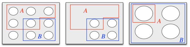
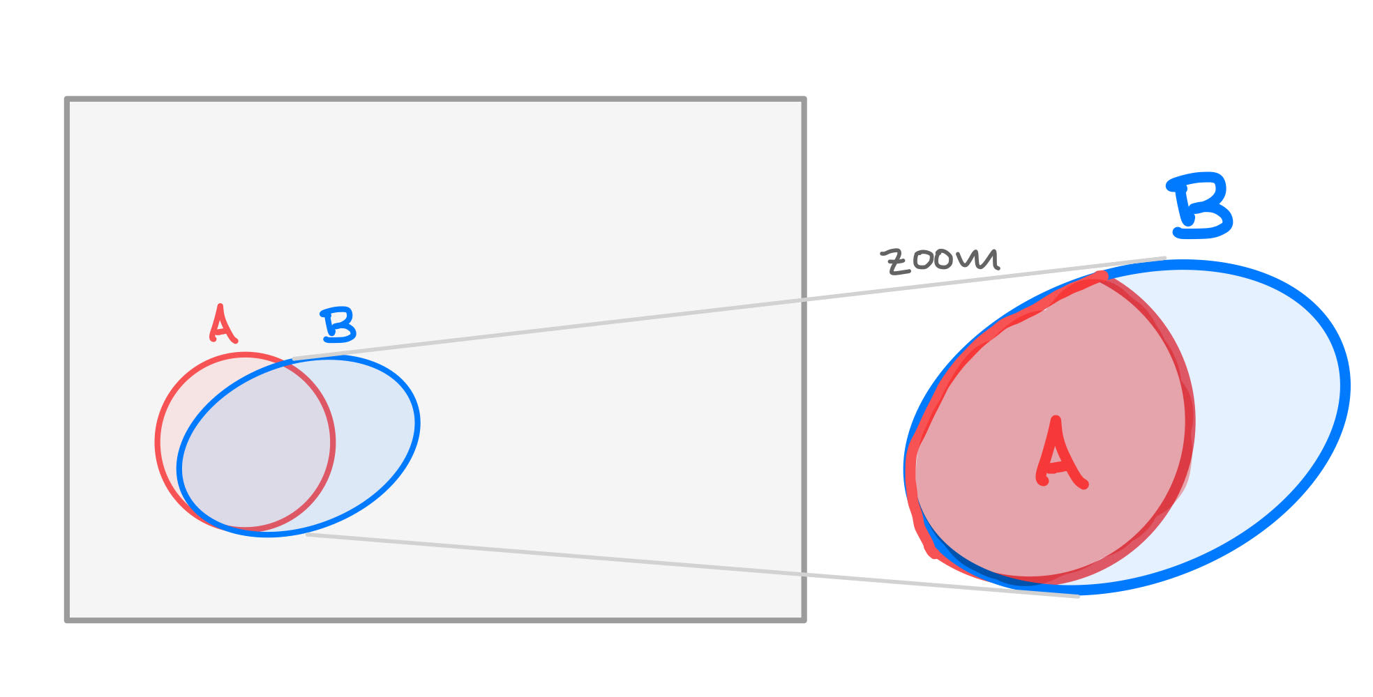
Zooming in on $B$. Image credit to Blitzstein and Hwang, chapter 2.

\[\Pr[A \mid B] = \frac{\Pr[A \cap B]}{\Pr[B]} = \Pr[B \mid A] \frac{\Pr[A]}{\Pr[B]}.\]

Failing to correctly account for conditional information is a very common source of mistakes in statistics and its applications! Today’s lecture is all about recognizing common mistakes in conditional logic.

Mistake 1: the base rate fallacy#

The base rate fallacy is the mistake of weighting specific information too heavily, without remembering the bigger picture.

If you like, this is the mistake of “conditioning too hard.”

Usually, people commit the base rate fallacy when:

They care about estimating $\Pr[A]$.
They are told that $B$ happens.
They know $\Pr[B \mid A]$ is large.
They mistakenly conclude that $\Pr[A \mid B]$ is also large.

What this chain of thought gets wrong is that if the base rate $\Pr[A]$ is really small, then $\Pr[A \mid B]$ can still be small.

In the base rate fallacy, people fail to take into account that $\Pr[A\mid B]$ could still be small, even though $\Pr[B \mid A]$ is large.

Example: false positive tests#

You get tested for a rare disease affecting 1% of the population, with a test that is 99% accurate. When the test comes back positive, you’re certain that you have the disease.

Question: why is this an example of the base rate fallacy?

Let $A$ be the event that you have the disease, let $B$ be the event that the test comes back positive.

Before getting tested, we can take your chance of having the disease to be the “base rate,” $\Pr[A] = 0.01$.

When you get back the test result, that is, when you know $B$ occurs, you feel certain that you have the disease, because it is a 99% accurate test.

But if we remember to take the base rate into account, as we saw in the last lecture,

\[ \Pr[A \mid B] = \Pr[B \mid A]\frac{\Pr[A]}{\Pr[B]} \]

\[ = \Pr[B \mid A]\frac{\Pr[A]}{\Pr[B \mid A]\cdot \Pr[A] + \Pr[B \mid \overline{A}] \cdot \Pr[\overline{A}]} \]

\[= 0.99 \cdot \frac{0.01}{0.99 \cdot 0.01 + 0.01 \cdot 0.99} = \frac{1}{2},\]

So when we remember the base rate, there is actually only a 50% chance that you have the disease, even conditioned on the information of the positive test.

Example: personality traits#

Remember the “is Steve more likely to be a librarian or farmer?” example from Monday?

Khaneman and Tversky wrote the influential article On the Psychology of Prediction in 1973, in which they studied peoples’ tendency to commit the base rate fallacy.

They did the following experiment: they had two groups, each with $n$ participants.

Group 1 was asked to respond to the following prompt:

There is a group of 30 engineers and 70 lawyers, and psychologists have made personality sketches of some of the group.
“Jack is a 45-year-old man. He is married and has four children. He is generally conservative, careful, and ambitious. He shows no interest in political and social issues and spends most of his free time on his many hobbies which include home carpentry, sailing, and mathematical puzzles. What is the probability that Jack is one of the 30 engineers in the sample of 100?”

The second group was given the same prompt, but the proportion of engineers and lawyers was flipped (so the majority were now lawyers).

There was effectively no difference between group 1 and 2 in the median probability assigned to the event that Jack is an engineer.

Question: why is this an example of the base rate fallacy?

Mistake 2: Conditioning out of context#

Sometimes you will hear a conditional probability which sounds impressively large (or small), without enough context to understand if conditioning increased or decreased the probability.

Did conditioning on $B$ increase the chance of $A$?

Or did it decrease the chance of $A$?

As far as I know this fallacy has no canonical name, but I will call it the fallacy of conditioning without context.

Example: second biggest state in the NFL#

You are told that the state home to the second-largest number of NFL players is California; 151 out of 1696 players are from California (about 9%).

Does being from California improve your chances of playing in the NFL?

Question: Can you phrase this question in the language of conditional probabilities?

Let $F$ be the event of playing in the NFL. Let $C$ be the event of being Californian.

We know that $\Pr[C \mid F] = 0.09$.

Now we want to know whether $\Pr[F \mid C] > \Pr[F]$?

To answer this question, we actually need to know what proportion of people are from California to begin with!

Why we need more context#

Fact: If $A,B$ are events, then $\Pr[A \mid B] > \Pr[A]$ if and only if $\Pr[B] < \Pr[B \mid A].$

This is because $\Pr[A \mid B] \cdot \Pr[B] = \Pr[A \cap B] = \Pr[B \mid A] \cdot \Pr[A]$.

So $\Pr[F \mid C] > \Pr[F]$ only if $\Pr[C] < \Pr[C \mid F]$.

In fact, being from California decreases your chances of playing in the NFL!

The population of California is $\approx$ 39 million. The population of the U.S. is 340 million.

So $\Pr[C] = 39/340 \approx 0.11 > \Pr[C \mid F]$.

Example: a male-dominated sport#

Here is an example from The Gaurdian, also covered in the news quiz show “Wait, wait, don’t tell me,” It’s the part about hiking in Scotland in the transcript here.

Of 114 Scottish hiking fatalities in the last decade, 104 were men. This suggests that male Scottish hikers are more reckless than female Scottish hikers.

Question: what is wrong with this reasoning? Phrase it in the language of conditional probability.

Let $M$ be the event that a hiker is male, and let $A$ be the event of a hiking accident.

The statistic above can be re-written as $$\Pr[M \mid A] = 104/114.$$

The mistake here is to then assume that $\Pr[A \mid M]$ must also be large, in fact larger than $\Pr[A \mid \overline{M}]$, i.e. “men are more reckless than women.”

But some sports are very male-dominated.

If the base rate $\Pr[M] = 104/114$, then the events $M$ and $A$ are actually independent!

And then $\Pr[A \mid M] = \Pr[A \mid \overline{M}]$.

Mistake 3: The prosecutor’s fallacy#

The prosecutor’s fallacy is the mistake of confusing the probability of evidence given innocence with the probability of innocence given the evidence.

Let $G$ be the event that the accused is guilty. Let $E$ be the event that the trial evidence is observed.

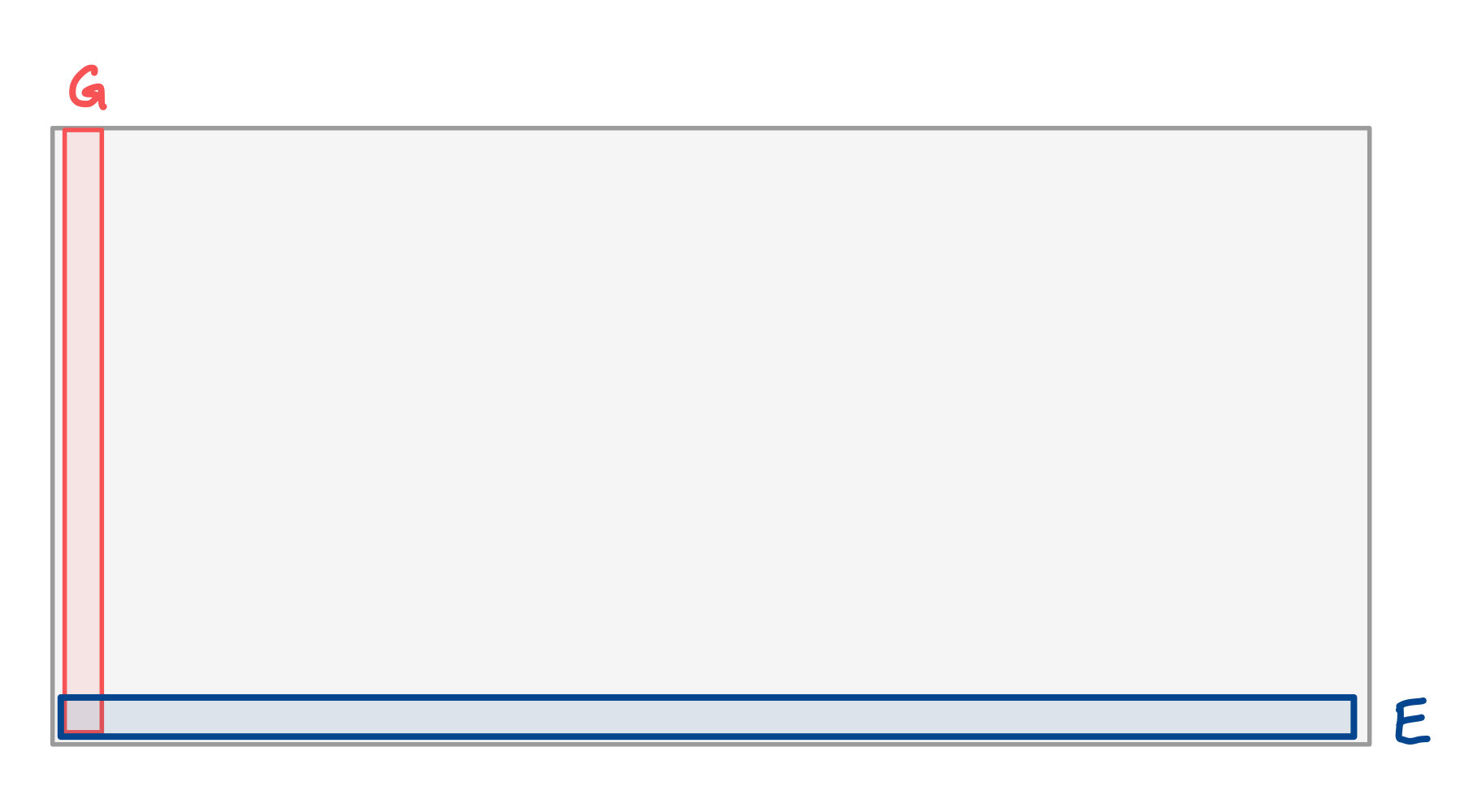
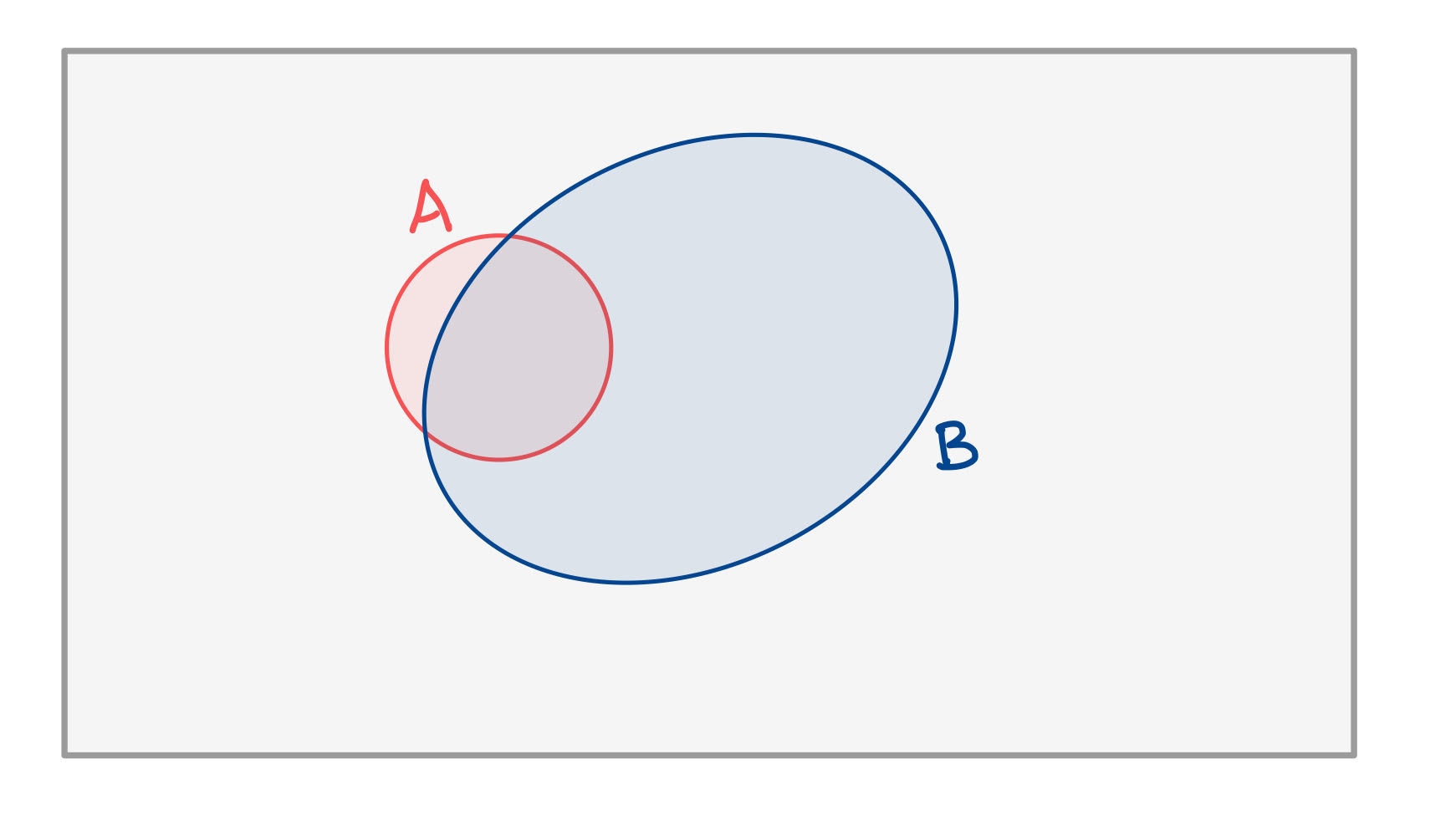
The prosecutor's fallacy says that when you condition on innocence (zoom in on $\overline{G}$), the evidence $E$ is very unlikely. But maybe the evidence is just unlikely, independent of $G$?

A common argument made by prosecutors is that the evidence is very unlikely, conditioned on innocence:

$\Pr[E \mid \overline{G}]= 0.01$

But this does not take into account the fact that guilt and/or the evidence itself might be extremely unlikely. If we properly compute the probability of innocence given the evidence,

\[\Pr[\overline{G} \mid E] = \Pr[E \mid \overline{G}]\frac{\Pr[\overline{G}]}{\Pr[E]}\]

\[= \Pr[E \mid \overline{G}]\frac{\Pr[\overline{G}]}{\Pr[E]}\]

A tricky aspect of this fallacy is that it is often hard or impossible to compute the probability of the evidence, $\Pr[E]$. But the point is that even when we cannot compute $\Pr[\overline{G} \mid E]$, the conditional logic used by the prosecution does not make sense.

Example: Sally Clark case#

In 1999, an English woman named Sally Clark is found guilty for the murder of her two infant sons; both sons tragically died in early infancy, 2 years apart.

Her defense was that both had died of Sudden Infant Death Syndrome (SIDS).

The prosecution argued that the chance of having two sons die of SIDS in the same family was $1$ in $73$ million.

This calculation is problematic on its own, because it is given by squaring the probability of having one child die of SIDS, which was taken to be 1/8500.

Question: what does the 1/73 million calculation assume? What’s wrong with this assumption?

Let $E$ be the event that two sons of the same mother die in infancy.

Let $G$ be the event that the mother is guilty of murdering both.

Suppose, for the sake of simplicity, that if the sons are not murdered, the only possible alternative explanation is SIDS.

The chance that two children in the same family die of SIDS is actually closer to

\[\Pr[E \mid \overline{G}] = 2.7 \times 10^{-6};\]

But really, we are interested in the chance Sally is innocent given the evidence,

\[\Pr[\overline{G} \mid E].\]

Using Bayes’ rule,

\[ \Pr[\overline{G}\mid E] = \Pr[E \mid \overline{G}] \cdot \frac{\Pr[\overline{G}]}{\Pr[E]}. \]

In the UK, the frequency at which two children in the same family are murdered by their mother is something like $\Pr[G] = 3.7 \times 10^{-7}$.

So $\Pr[\overline{G}] = 1 - 3.7 \cdot 10^{-7} \approx 1$.

Plugging in to Bayes’ rule, $$ \Pr[\overline{G}\mid E] = \Pr[E \mid \overline{G}] \cdot \frac{\Pr[\overline{G}]}{\Pr[E]}$$= \Pr[E \mid \overline{G}]\cdot \frac{\Pr[\overline{G}]}{\Pr[E\mid G]\cdot \Pr[G] + \Pr[E \mid \overline{G}] \cdot \Pr[\overline{G}]}$$= 2.7 \times 10^{-6} \cdot \frac{1-3.7 \times 10^{-7}}{1\cdot 3.7 \times 10^{-7} + 2.7 \times 10^{-6} \cdot (1-3.7 \times 10^{-7})}$$ <font color="maroon">$$\approx 0.88.$$

Question: what is the problem with the prosecution’s logic?

The problem with the prosecution’s logic is that it does not take into account how rare murder is, nor how rare it is to have two infant deaths in the same family!

Mistake 4: The defense attorney’s fallacy#

The defense attorney’s fallacy is the mistake of failing to condition on all of the available information.

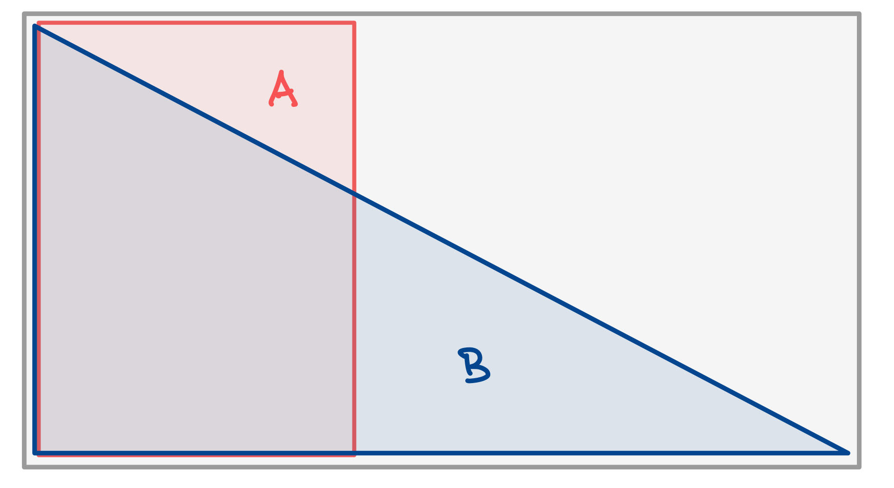
The defense attorney's fallacy: A is not likely. But when you condition on B, it becomes quite likely.

The OJ Simpson trial example that we have already seen is a great example.

Example: optimistic study habits#

“Only 1 in 10 students fail their qualifying exam, so I don’t need to study hard for it.”

Question: Why is this an example of the defense attorney’s fallacy? Can you put it in the language of conditional probabilities?

Mistake 5: Generalizing from a biased sample#

A final mistake is to mistake a conditional probability with an unconditioned probability. This is basically sample bias.

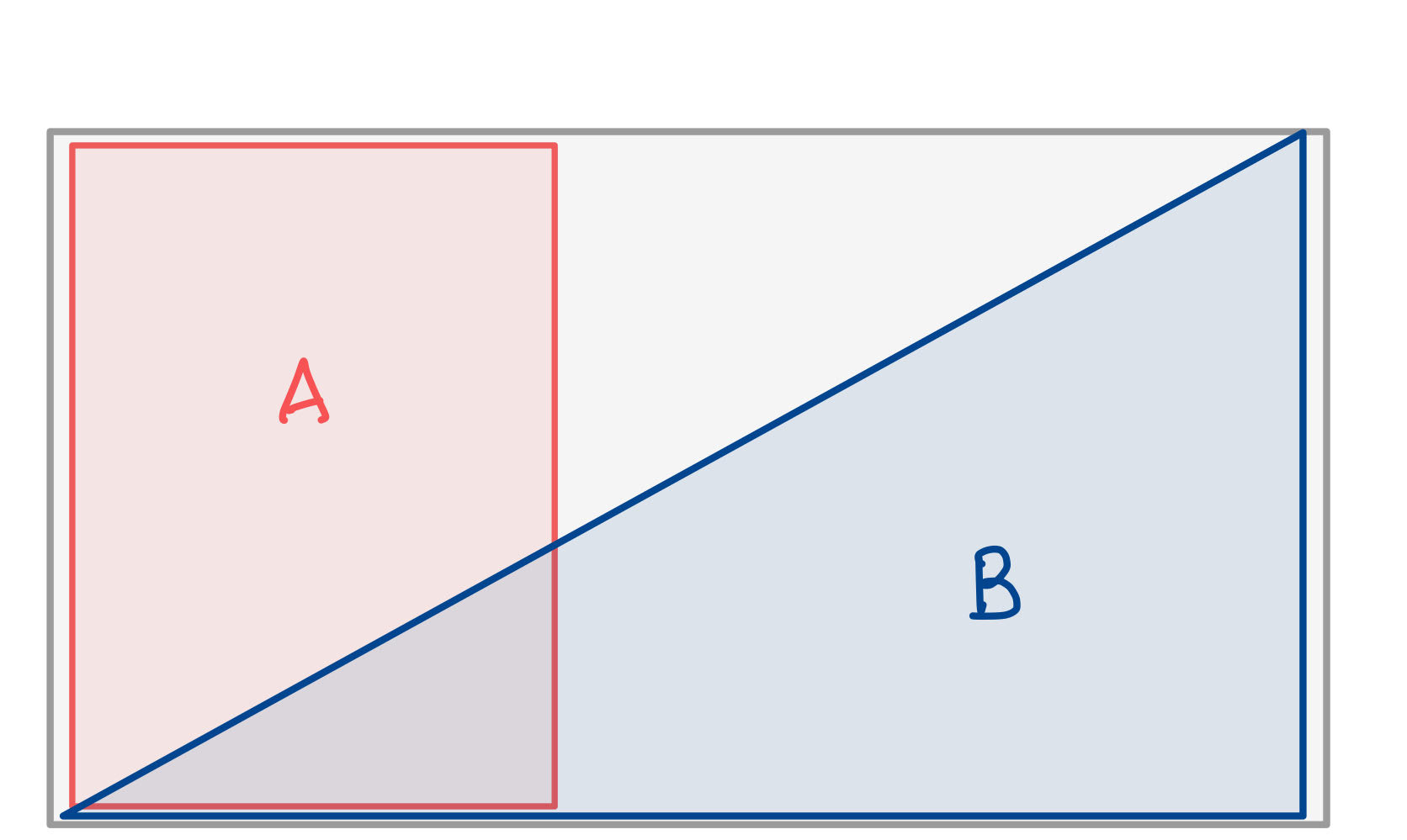
The idea is that you observe $\Pr[A \mid B]$ where $B$ is your biased sample. But really you want to know $\Pr[A]$.

You only observe $\Pr[A \mid B]$, and then take that as a good estimate of $\Pr[A]$. But what about $\Pr[A \mid \overline{B}]$?

It is like the defense attorney’s fallacy, but in reverse!

Example: hot guys are jerks!#

This example taken from Jordan Ellenberg and Calling Bullshit, chapter 6.

You might hear your friends on the dating scene complain that hot guys are jerks.

Let $J$ be the event that a man is a jerk, and let $H$ be the event that the man is hot.

Question: In the language of conditonal probabilities, what are your friends saying?

\[\Pr[J \mid H] > \Pr[J].\]

But this could just be an artefact of sample bias! Let $D$ be the event that your friend dated the guy. Really what your friend knows is that

\[\Pr[J \mid H \cap D] > \Pr[J].\]

Could it be that the men in your friends’ dating pool who are hot are also jerks, because of sample bias?

Consider the following explanation: it is possible that in the dating pool of guys, hotness and kindness are unrelated.

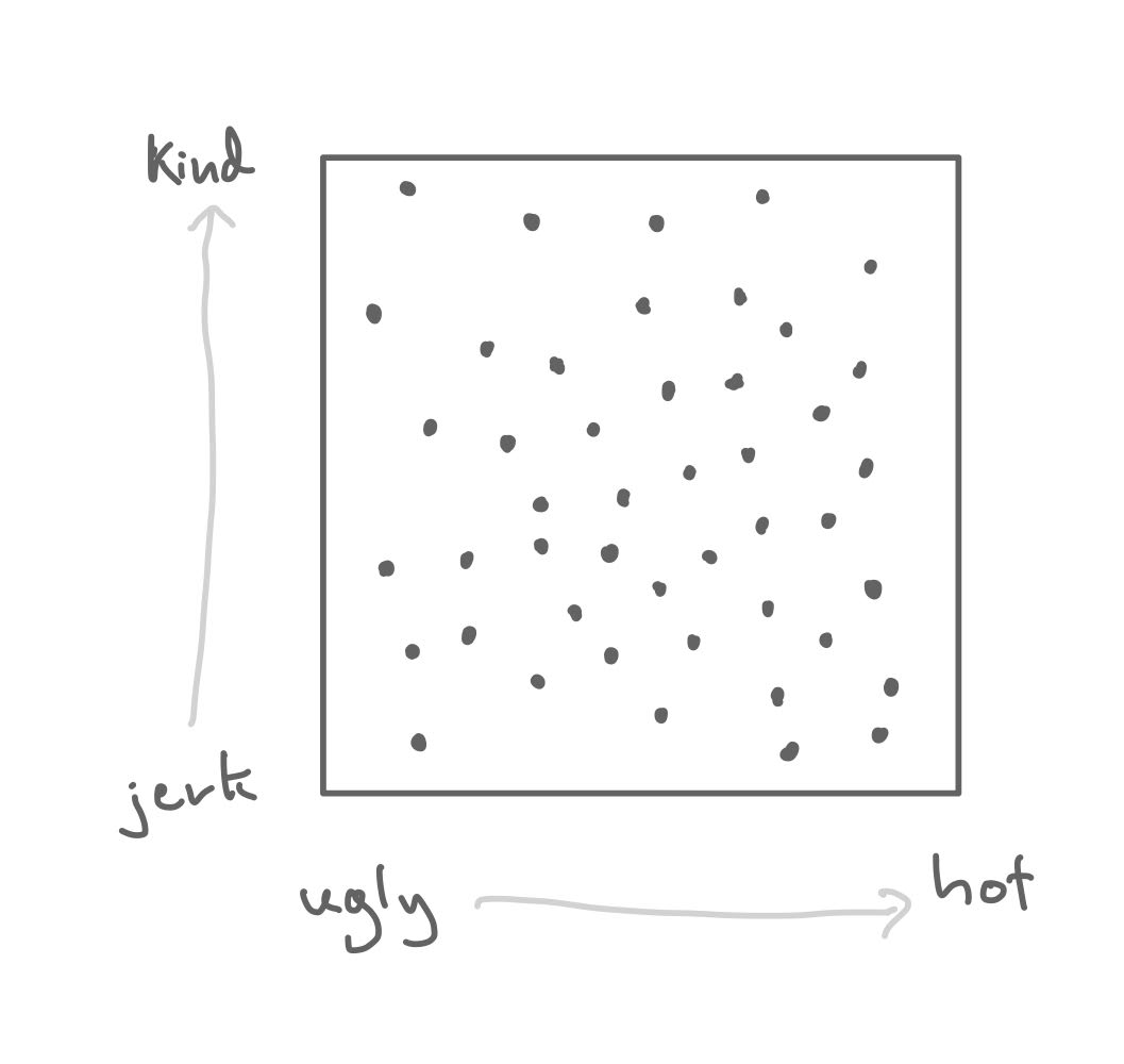
The dating pool of guys: a sample space.

But your friend has standards: they are unwilling to consider someone who is both ugly and a jerk. They would never even consider dating someone who is both ugly and a jerk.

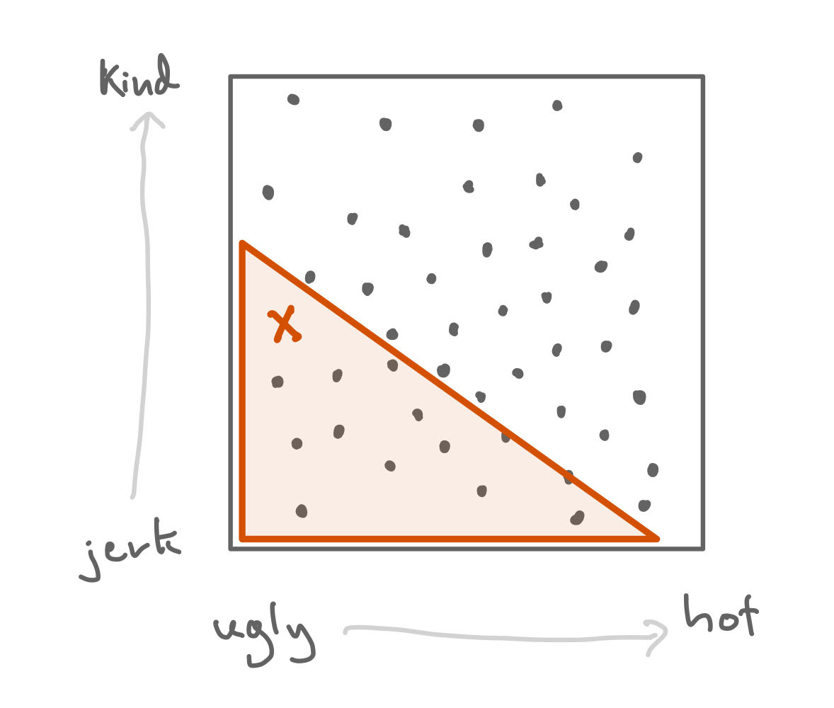
The event X, that someone is both ugly and a jerk, eliminates the guy from your friends' dating pool.

Similarly, the hottest, kindest guys might be already taken, and/or out of your friends’ league.

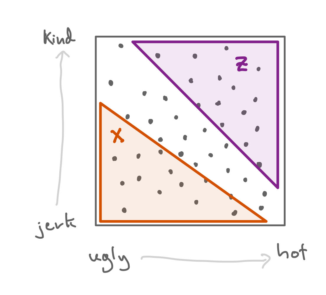
The event Z, that someone is extremely kind and hot, means they are probably already taken.

But then, within your friend’s dating pool, it might be the case that hot guys are more likely to be jerks!

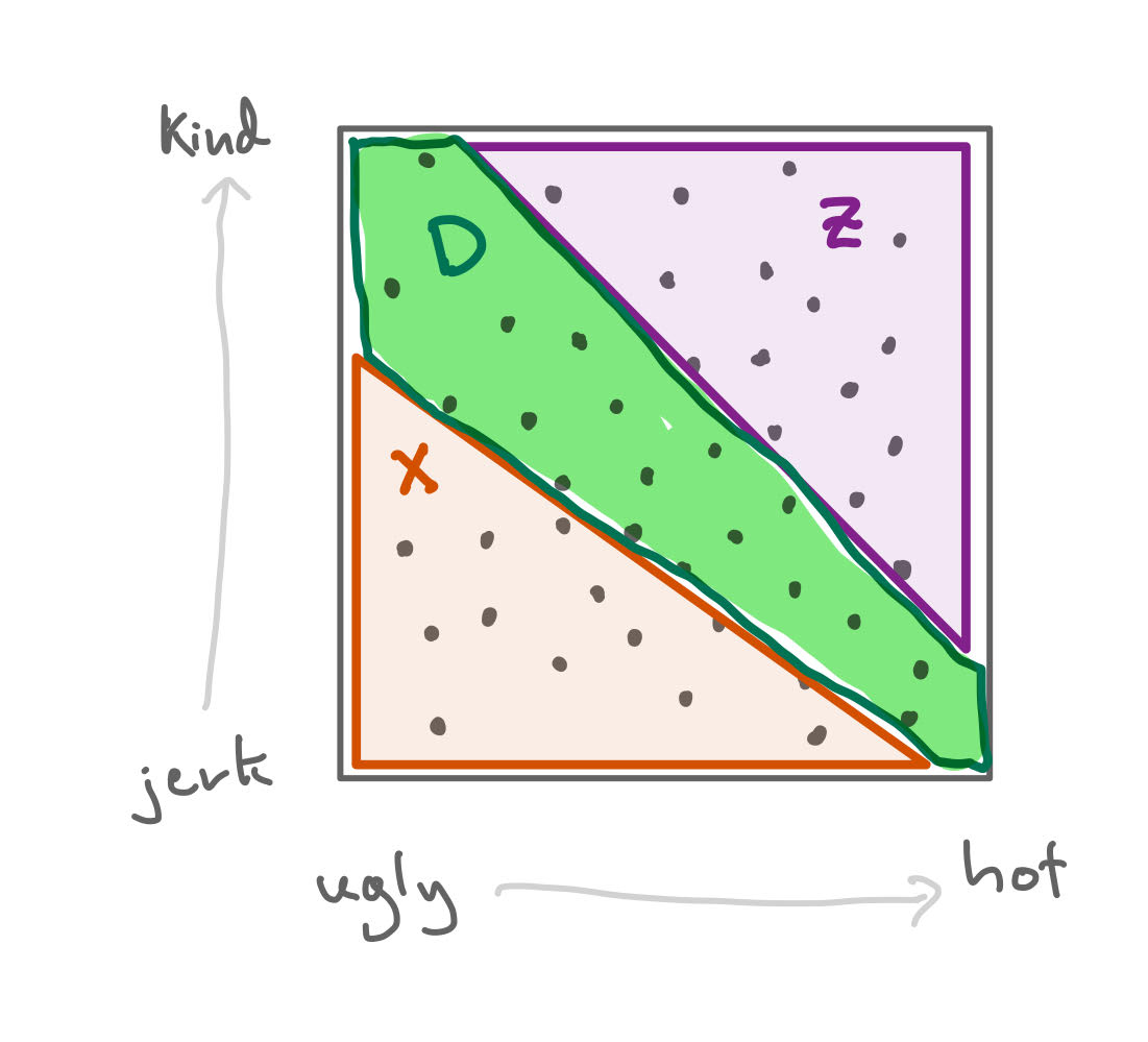
The event D is your friends' dating pool.