Lecture 12: Summaries of Center#
STATS 60 / STATS 160 / PSYCH 10
USA Women’s Eight Rowing#
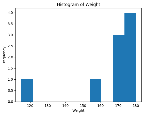
Shown below are stats for the members of the USA Women’s Eight rowing team that competed at the 2024 Paris Olympics.
Histogram#
For a quantitative variable like Weight, we can use a histogram to
visualize the distribution of the data.
But what if we wanted to summarize the data by a single number?
Mean#
One common summary of a quantitative variable is the mean (or average, although this is less precise).
To calculate the mean, add up the numbers and divide by how many there are: $\( \bar x = \text{mean} = \frac{x_1 + x_2 + \dots + x_n}{n}. \)$
Calculate the mean weight of the rowers.
When do you think was the first time in history that someone computed a mean to summarize data?
Answer: Not until about 1720!
Interpreting the Mean#
The mean \(\bar x \approx 166.7\) measures the “center” of the distribution.
It is where the histogram would “balance” if we put it on a scale.
Median#
The mean is not the only way to summarize the center of a distribution. Another summary is the median, the middle value when the data is sorted in order.
Calculate the median weight of the rowers.
When \(n\) is even, there are two middle numbers. The median is the mean of the two middle numbers.
Calculate the median weight of the \(n=8\) rowers, excluding the coxswain.
Interpreting the Median#
The median \(170\) is another summary of the “center” of the distribution.
It is the value where half the data is below and half the data is above.
Mean vs. Median#
We have now seen two different summaries of center:
\(\displaystyle \text{mean} = \frac{170 + 180 + 115 + 170 + 175 + 170 + 180 + 180 + 160}{9}\)
\(\displaystyle 115, 160, 170, 170, \underbrace{170}_{\text{median}}, 175, 180, 180, 180\)
What would happen to the mean and median if the coxswain weighed only 90 pounds? What if the coxswain weighed 140 pounds?
Answer: The mean would change, but the median would not.
Moral: The mean is sensitive to outliers (in either direction), but the median is not. Statisticians say that the median is more “robust” than the mean.
Exercise#
Shown below is a histogram of the arrival delays from the flights data.
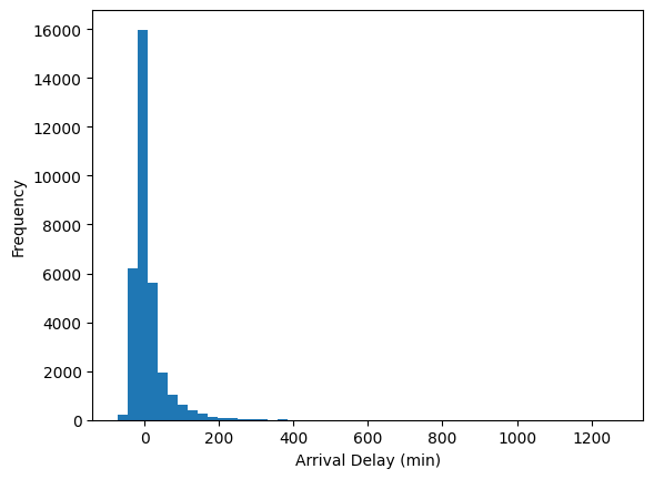
How do you think the mean and median of the arrival delays compare?
\(\text{mean} \approx 7.1\)
\(\text{median} = -5.0\)
#
The Center Doesn’t Tell the Whole Story#
Many people think that the mean/median represent the “typical” value, but this is not always the case.
Consider the Old Faithful eruption times from last class.
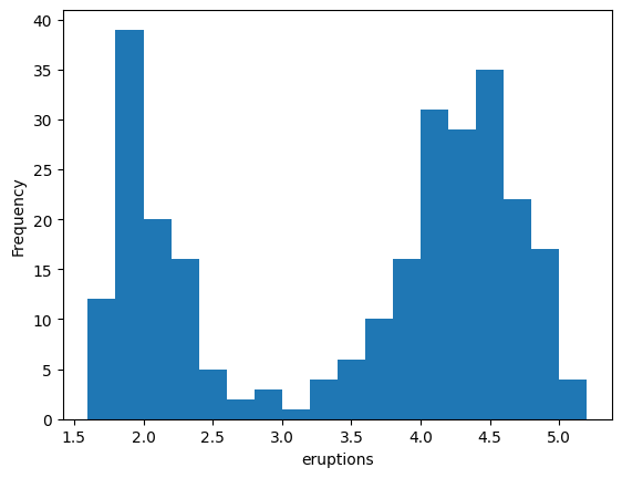 The mean eruption time is about \(3.5\) minutes.
If we only reported this number, we would miss the fact that most eruptions are either much shorter or much longer!
Variability#
Shown below are histograms of daily average temperatures in two cities.
Chicago
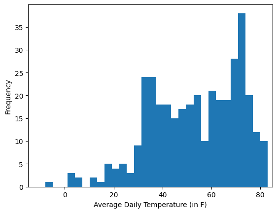 Seattle
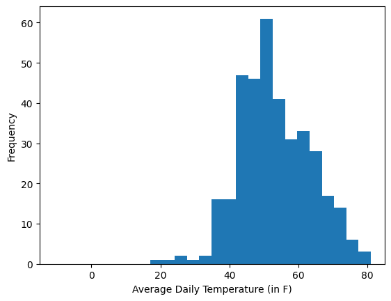
The means of the two cities are about the same (\(53.25^\circ\text{F}\) for Chicago vs. \(53.07^\circ\text{F}\) for Seattle), but the distributions are very different.
Recap#
The mean and the median are two summaries of center.
The median is more robust to outliers.
However, summaries of center don’t paint the full picture.
Next class: summaries of variability