Lecture 17: The Normal Approximation

STATS 60 / STATS 160 / PSYCH 10

Concepts and Learning Goals:

• Confidence intervals

  • Larger sample size implies better confidence intervals

• The Normal approximation

  • Central Limit Theorem

  • 68-95-99 rule

The sample mean

Remember our setup from Monday:

0. We have a population of size \(N\), each member has a feature described by a variable \(x\), we are trying to measure \(\mu\), the population mean of \(x\)

1. We take a uniform sample of size \(n\) from the population and measure the variable values $\( x_1,\ldots,x_n.\)$

2. We compute the sample mean \(\hat\mu_n = \bar{x} = \frac{x_1+\cdots+x_n}{n}\) as an estimate for \(\mu\).

We learned on Monday that our estimate \(\hat\mu_n\):

• Is a random quantity, because the value depends on the random sample

• The expectation of the sample mean is the population mean, \(\mathbb{E}[\hat\mu_n] = \mu\)

• Has standard deviation \(\frac{1}{\sqrt{n}}\sigma_x\), where \(\sigma_x\) is the population standard deviation of \(x\).

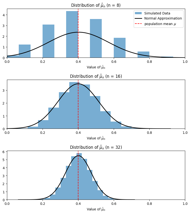
The Normal Approximation

In the setting of sampling from a population, something profoundly amazing happens:

No matter what the population or the variable \(x\) are, when \(n\) is large enough, the distribution of \(\hat\mu_n\) becomes close to the Normal Distribution!

The Normal Distribution

The Normal Distribution is a specific type of distribution which looks like this:

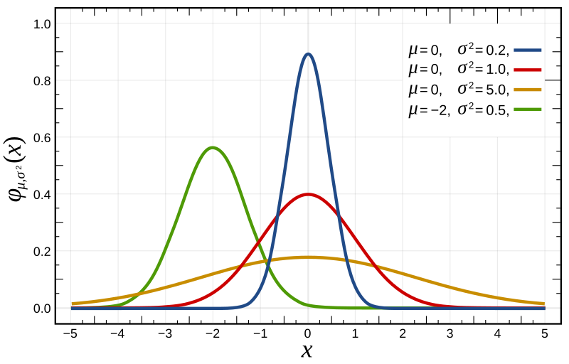
Image from Wikipedia.

It is also called the Gaussian Distribution or the Bell Curve.

The definition of the Normal distribution is, more or less, the distribution of the sample average when \(n\) is really big.

Incredibly: the only details of the population that influence the (large \(n\) limiting) distribution of \(\hat\mu_n\) are the population mean \(\mu\) (which dictates where the distribution is centered) and the population variance \(\sigma^2\) (which dictates the variability).

Why? The Central Limit Theorem; understanding its proof requires only a bit of background in probability. I prove it in lecture when I teach STATS 116 (or 118).

Accuracy of our estimates?

Remember that we had several different scenarios where we wanted to get an estimate:

• The hot dog poll

• Palo Alto water microplastics concentration measurement

• Measuring average duration of headache side effects

In all three of these, we made an estimate for the quantity \(\mu\) that we cared about using the sample mean \(\hat\mu_n\).

We want to know:

• How accurate is \(\hat\mu_n\)?

• How unlikely is it that our error is large?

  • What is the probability that \(|\hat\mu_n - \mu| > \frac{1}{10}\)?

Normal approximation gives us approximate probability of error

In the hot dog poll, we could exactly compute the probability that \(|\hat\mu_n - \mu| > \frac{1}{10}\) using coinflips.

In the microplastics/medicine side effects scenarios, that seems hard or impossible!

• How would we model microplastic concentration in water samples with coins/dice/marbles?

• We might be able to make something work for headaches, but it would be annoying.

Because of the Central Limit Theorem we know that, when \(n\) is big enough, \(\hat\mu_n\) is effectively Normally distributed!

This gives us a way to calculate \(\Pr[|\hat\mu_n - \mu|>\frac{1}{10}]\): use the Normal distribution!

Confidence intervals

Now we introduce the concept of a confidence interval, which allows us to directly reason about the error of our estimate, \(|\hat{\mu_n} - \mu|\).

How sure and how close?

Say \(\mu\) is an unknown quantity and \(\hat{\mu}\) is a random estimate of \(\mu\).

We want quantitative terminology for the idea that

“We are pretty sure that \(\hat{\mu}\) is close to \(\mu\).”

There are two quantities we need to specify:

1. How sure?

2. How close?

We use the term “confidence” to describe how sure we are.

To describe how close we are, we give an “interval” around our estimate which contains the true quantity.

Confidence intervals

“We are pretty sure (confident) that \(\hat{\mu}\) is close to \(\mu\) (\(\mu\) is in an interval/window around \(\hat{\mu}\)).”

We say that the interval \([\hat{\mu}-a ,\hat{\mu} + a]\) is a \(1-\alpha\) confidence interval for \(\mu\) if

\[ \Pr[ |\hat{\mu} - \mu| \le a ] \ge 1-\alpha, \]

that is, \(\mu\) is between \(\hat\mu - a\) and \(\hat\mu + a\) with probability at least \(1-\alpha\).

We can also have an asymmetric confidence interval: $[\hat{\mu}-b ,\hat{\mu} + a]$ is a $1-\alpha$ confidence interval for $\mu$ if

\[ \Pr[ a \le \hat{\mu} - \mu \le b ] \ge 1-\alpha, \]

that is, \(\mu\) is between \(\hat\mu - b\) and \(\hat\mu + a\) with probability at least \(1-\alpha\).

Practice with confidence intervals

Consider the distribution over \(\hat{\mu}\) defined by the following histogram:

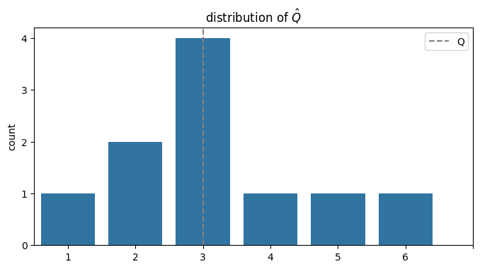
Question:

1. What is the confidence level for the interval \([\hat{\mu} - 1, \hat{\mu} + 1]\)?

   • That is, what is the probability that \(|\hat{\mu} - \mu| \le 1\)?

2. What is the size \(a\) of the confidence interval with confidence \(0.8\)?

   • That is, how large do we need to take \(a\) so that \(\Pr[|\hat{\mu}-\mu| \le a] \ge 0.8\)?

Sample size and confidence intervals

Let’s see how the confidence intervals change with \(n\).

I wrote some code to simulate this; here’s the code just in case you are curious.

# Code that computes the confidence for the interval mu +/- 0.1
# And finds the size of the 0.9-confidence interval.
import matplotlib.pyplot as plt
import random
T = 10000
mu = 43/107
Class = [1] * 43 + [0] * (107 - 43) # Make a list of "students" in the class; 1's are hot dog = sandwich people
Estimates = [0]*T
def confidence(n, plot=True):
    Estimates = [0]*T
    for t in range(T): # Run T independent polls
        X = random.sample(Class,n) # Survey n students each time
        Estimates[t] = sum(X)/n    # Record \mu_n

    # confidence of interval with size 0.1:
    conf = sum(1 for x in Estimates if abs(x-mu) < 0.1)/T 

    # size of interval with confidence 0.9:
    Diffs = [abs(hmu - mu) for hmu in Estimates]
    Diffs.sort()
    size = Diffs[T*9//10]
    
    if plot:
        plt.hist(Estimates, bins=15) # Plot a histogram of the data 
        plt.xlabel('Estimate of $\mu$')
        plt.title('Variability in estimate of $\mu$, n ='+str(n))
        plt.axvline(x=mu, color='red', linestyle='--', linewidth=1)
#        plt.axvline(x=mu - 0.1, color='black', linestyle='--', linewidth=2,label='confidence for 0.1-sized interval = '+str(conf))
#        plt.axvline(x=mu + 0.1, color='black', linestyle='--', linewidth=2)
        plt.axvline(x=max(0,mu - size), color='blue', linestyle='--', linewidth=2, label='.9-confidence interval')
        plt.axvline(x=mu + size, color='blue', linestyle='--', linewidth=2)
        plt.xlim(-.1,1)
        plt.legend()
        plt.show()
    return (size,conf)

N = 50
confs = [0]*N
sizes = [0]*N
for n in range(2,N):
    (a,g)=confidence(n,False) 
    confs[n] = g
    sizes[n] = a

<>:25: SyntaxWarning: invalid escape sequence '\m'
<>:26: SyntaxWarning: invalid escape sequence '\m'
<>:25: SyntaxWarning: invalid escape sequence '\m'
<>:26: SyntaxWarning: invalid escape sequence '\m'
/tmp/ipykernel_29930/996443862.py:25: SyntaxWarning: invalid escape sequence '\m'
  plt.xlabel('Estimate of $\mu$')
/tmp/ipykernel_29930/996443862.py:26: SyntaxWarning: invalid escape sequence '\m'
  plt.title('Variability in estimate of $\mu$, n ='+str(n))

---

Smallest sample, \(n = 2\).

confidence(2)

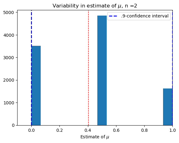
(0.5981308411214954, 0.4818)

---

Small sample, \(n = 4\).

confidence(4)

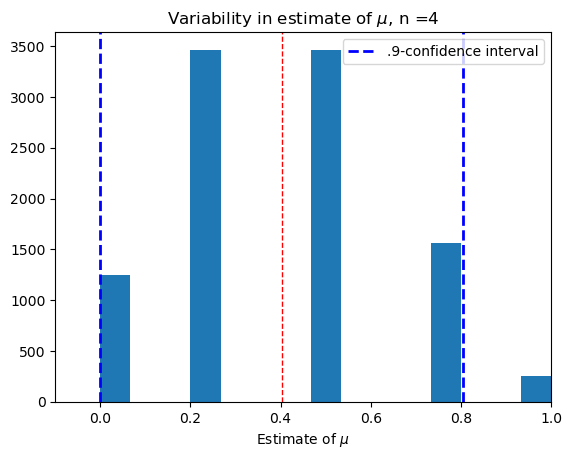
(0.40186915887850466, 0.359)

---

Medium-small sample, \(n=8\).

confidence(8)

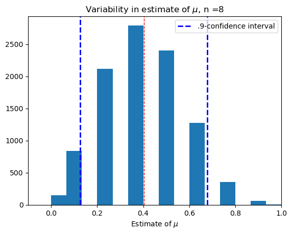
(0.27686915887850466, 0.5384)

---

Medium sample, \(n = 16\).

confidence(16)

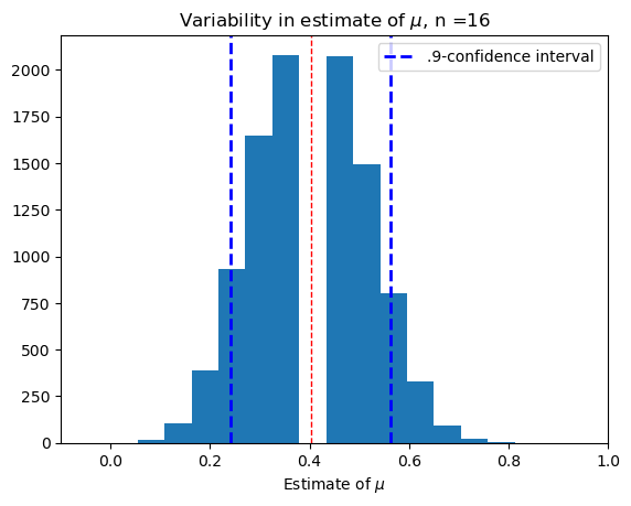
(0.16063084112149534, 0.7334)

---

Largeish sample, \(n = 32\).

confidence(32)

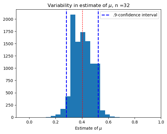
(0.12061915887850466, 0.8646)

---

Large sample, \(n = 64\)

confidence(64)

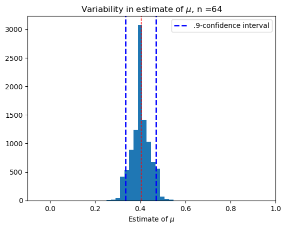
(0.06688084112149534, 0.9909)

---

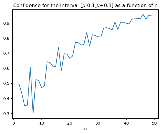
Larger samples give higher confidence

What is the probability that \(|\hat{\mu}_n - \mu| \le \frac{1}{10}\) for each \(n\)?

Put another way, what is our confidence level for the interval \((\hat{\mu_n}-\frac{1}{10},\hat{\mu_n}+\frac{1}{10})\)?

plt.plot(range(2,N), confs[2:])
plt.title('Confidence for the interval [$\mu$-0.1,$\mu$+0.1] as a function of n')
plt.xlabel('n')
plt.show()

<>:2: SyntaxWarning: invalid escape sequence '\m'
<>:2: SyntaxWarning: invalid escape sequence '\m'
/tmp/ipykernel_29930/711082639.py:2: SyntaxWarning: invalid escape sequence '\m'
  plt.title('Confidence for the interval [$\mu$-0.1,$\mu$+0.1] as a function of n')

---

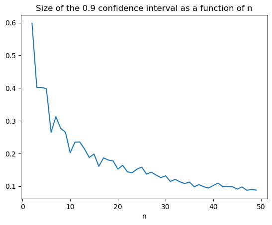
Larger samples give smaller intervals

How small can we take \(a\) if we want to make sure that \(\Pr[|\hat{\mu}_n - \mu| \le a] \ge 0.9\) for each \(n\)?

Put another way, what is the size of the \(0.9\)-confidence interval for \(\mu\) around \(\hat{\mu_n}\)?

plt.plot(range(2,N), sizes[2:])
plt.title('Size of the 0.9 confidence interval as a function of n')
plt.xlabel('n')
plt.show()

Sample mean confidence intervals from the Normal Approximation

The 68-95-99 rule

If \(Z\) is Normal with mean \(\mu_Z\) and variance \(\sigma_Z^2\), then:

1. \(\Pr[|Z-\mu_Z| \le \sigma_Z] \approx .68\).

2. \(\Pr[|Z-\mu_Z| \le 2\sigma_Z] \approx .95\).

3. \(\Pr[|Z-\mu_Z| \le 3\sigma_Z] \approx .997\).

Confidence Intervals for the sample mean

In the scenario of estimating \(\mu\) with the sample mean \(\hat{\mu_n}\), as long as \(n\) is large enough, the sample mean is close to Normally distributed with mean \(\mu\) and variance \(\sigma_x^2/n\).

Image from [Wikipedia

So as long as \(n\) is large enough: the sample mean \(\hat{\mu_n}\) is within

1. \(\frac{\sigma}{\sqrt{n}}\) of \(\mu\) \(68\%\) of the time,

2. Within \(\frac{2 \sigma}{\sqrt{n}}\) of \(\mu\) \(95\%\) of the time,

3. Within \(\frac{3 \sigma}{\sqrt{n}}\) of \(\mu\) \(99.7\%\) of the time.

Practice with sample mean confidence intervals

Using the 68-95-99 rule: if \(n\) is large enough, then \(\hat\mu_n\) is

1. Within \(\frac{\sigma}{\sqrt{n}}\) of \(\mu\) \(68\%\) of the time,

2. Within \(\frac{2 \sigma}{\sqrt{n}}\) of \(\mu\) \(95\%\) of the time,

3. Within \(\frac{3 \sigma}{\sqrt{n}}\) of \(\mu\) \(99.7\%\) of the time.

Let’s practice with the hotdog poll:

How large should \(n\) be?

1. How large should I take \(n\) to be 95% sure that my estimate is within \(\frac{1}{10}\) of the truth?

   • For 95% confidence, I need that \(2\frac{\sigma_x}{\sqrt{n}} \le \frac{1}{10}\).

   • I solve: \(n \ge (2 \sigma_x \cdot 10)^2 = 400 \sigma_x^2\).

   • To get a lower bound on \(n\), I need to know how large \(\sigma_x\) can be.

     Fact: In any yes/no poll situation, \(\sigma \le 1\).

     That’s because Fact: The standard deviation for variable \(x\) is always at most \(\sigma \le x_{\max} - x_{\min}\).

     We can actually improve this a little bit, in any yes/no poll, to \(\sigma \le \frac{1}{2}\).

   • So we need \(n \ge 400 \cdot \left(\frac{1}{2}\right)^2 = 100\)

If \(n\) is given

2. I was only able to poll \(n = 49\) people. How confident am I that I am within \(\frac{1}{10}\) of the truth?

   • We want to know how many standard deviations \(\frac{1}{10}\) is.

   • Solve for \(C\):

     \[\frac{1}{10} = C \cdot \frac{\sigma}{\sqrt{n}} = C \frac{\sigma}{\sqrt{49}} = \frac{C\sigma}{7}\]
     \[ C = \frac{7}{10\sigma} \ge \frac{14}{10}\]

   • \(C\) is between 1 and 2, so I am between \(68\%\) and \(95\%\) confident.

3. I only polled \(n = 49\) people. What is the error \(a\) for my \(95\%\) confidence interval?

   • Solve for $\( a = \frac{2\sigma}{\sqrt{n}} = 2 \frac{\sigma}{7} \le \frac{1}{7}}.\)$

In general

If I want to know how many samples I need to estimate \(\mu\) up to \(\epsilon\) with \(95\%\) confidence:

• Solve for the smallest \(n\) which gives \(\epsilon \ge 2\frac{\sigma}{\sqrt{n}}\): $\(n \ge \frac{4\sigma^2}{\epsilon^2}\)$

• Plug in your best upper bound on \(\sigma\).

  • What if I don’t know \(\sigma\)?

  • You can always substitute the range of \(x\): \(\sigma_x \le x_{\max} - x_{\min}\). This gives you a valid bound, but it could be pretty large.

  • You can estimate it from data (compute the standard deviation of your dataset).

Practice with Microplastics

Suppose I know \(\sigma_x = 10\).

1. How large should I take \(n\) to be 99% sure that my sample mean is within \(\frac{1}{10}\) of the true microplastics concentration?

   • To be \(99\%\) confident, we need an error of magnitude \(3\) times the standard deviation of the sample mean.

   • Since target error is \(\frac{1}{10}\), we need \(\frac{1}{10} \ge 3 \frac{\sigma_x}{\sqrt{n}} = 30/\sqrt{n}\).

   • Solving for \(n\), it’s sufficient to take \(n \ge (300)^2= 90,000\).

2. Suppose I only took \(n = 25\) samples. What is the size \(a\) of the error for my \(68\%\) confidence interval?

   • The size of error for the \(68\%\) interval is one standard deviation of the sample mean.

   • That means we need to solve for \(a = \frac{\sigma_x}{\sqrt{n}} = \frac{10}{\sqrt{25}} = 2\).

AI can help you compute confidence intervals.

I think GPT and other chat interfaces are still a bit unreliable if you ask them straight-up. But if you ask them to write code to do it, they’re pretty good.

Let’s try Colab.

How large should \(n\) be for the Normal Approximation to kick in?

This question is totally separate from the question of how large should \(n\) be to make the confidence interval of size \(\le \epsilon\).

It depends on the variability/skew of the population distribution.

• A good rule of thumb is \(\min(np,n(1-p)) \ge 10\) for a scenario modeled by coin flips with heads probability \(p\).

• This means \(n \ge 20\) for fair coin flips. For coinflips that come up heads \(\frac{1}{3}\) of the time, \(n \ge 30\).

• If you use an \(n\) which is too small, your confidence intervals will be small and it is invalid to use the Normal Approxiation to calculate them!

Recap

• The sample mean approximately follows the Normal distribution when \(n\) is large enough.

• Confidence intervals give us a way to say how sure we are that an estimate is close to the ground truth

• Larger sample size \(\implies\) smaller confidence intervals & more confidence

• We can compute confidence intervals for the sample mean using the Normal approximation

  • The 68-95-99 rule

  • Use AI (a programming-based prompt is safest).