Lecture 21: Testing for Correlation

Lecture 21: Testing for Correlation#

STATS 60 / STATS 160 / PSYCH 10

Announcement:

Next week, guest lectures by Aditya and Prof Sun.
Randomized control trials!

Concepts and Learning Goals:

Hypothesis test for correlations
- testing via simulation
- permutation test
Estimating variability of correlation
- simulation: “The bootstrap”
- Bootstrap confidence intervals

Trends in multiple variables#

Until now we have been hypothesis testing for trends in a single variable:

AI vs. not photo challenge: proportion of correct guesses (the variable is $x_i = 0/1$, depending on whether guess is right)
Discrimination against North Americans: proportion of North Americans (the variable is $x_i = 0/1$, depending on whether the employee is North American)
Gettysburg address: length of word sampled (the variable is $x_i = \text{word length}$)

Many times, we measure multiple variables, and we want to test for a trend in how they are associated.

“Can variable $x$ actually help you predict variable $y$?”

Correlation#

Suppose that I have sampled $n$ individuals from my population, and for each I have measured the values $(x_i,y_i)$.

For example:

Penguins: $x =$ body mass, $y=$ beak length
Medicine: $x=$ blood pressure, $y=$ age
Economics: $x=$ years of education, $y=$ salary
College admissions: $x=$ SAT score, $y=$ sophomore-year GPA

The correlation coefficient of $x$ and $y$ is the slope of the best-fit line for the standardized datasets $x_1,\ldots,x_n$ and $y_1,\ldots,y_n$.

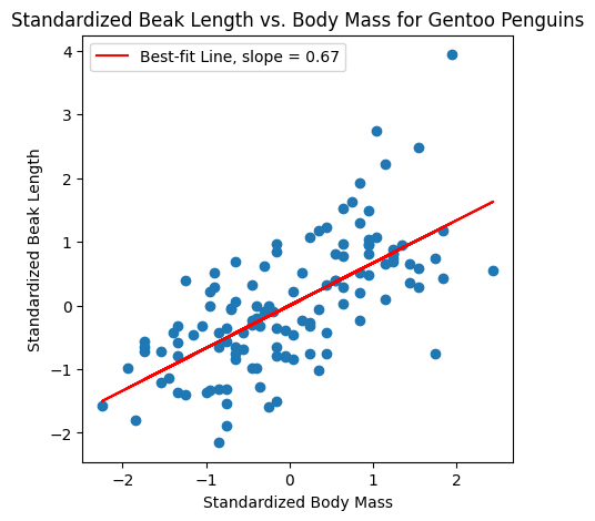
Correlation coefficient for Penguin body mass vs. beak length

\[ \text{correlation coefficient} = \hat R_{n} = \frac{1}{n}\sum_{i=1}^n \frac{(x_i - \bar{x})(y_i-\bar{y})}{\sigma_x \sigma_y }, \]

where $\bar{x},\sigma_x$ are the mean and standard deviation of the $x$’s, and $\bar{y},\sigma_y$ are the mean of and standard deviation of the $y_i$’s.

Variability in the correlation coefficient#

Usually, we want to know the population value of the correlation coefficient: the ground truth value $R$ across the whole population.

The correlation coefficient of our sample, $\hat R_{n}$, is a function of our sample data, so it is random, and exhibits variability.

If we got a different sample, we could get a different value of the correlation coefficient.

Suppose that we compute the correlation coefficient for our sample, and see that it has value $\hat R_n$.

If $\hat R_n \neq 0$, is this a sign of an actual association, or is it just a coincidence?
How much variability is there in $\hat{R}_n$?

Testing for correlation#

Suppose that we compute the correlation coefficient for our sample, and see that it has value $\hat R_n \neq 0$.

Is this just a coincidence? Or is the correlation a real pattern?

Let’s formulate this as a hypothesis testing problem:

Null Hypothesis: there is no correlation.
How can we compute the $p$-value?
- We’ll use simulation!
- FYI: if you are willing to make assumptions about the distributions of $x,y$ under null, you can use a Chi-squared ($\chi^2$) test (outside the scope of this STATS60).

Permuting the datapoints#

Let’s assume, from now on, that our $x_i$ and $y_i$ are standardized.

Suppose there really is a positive association between $(x_i,y_i)$.

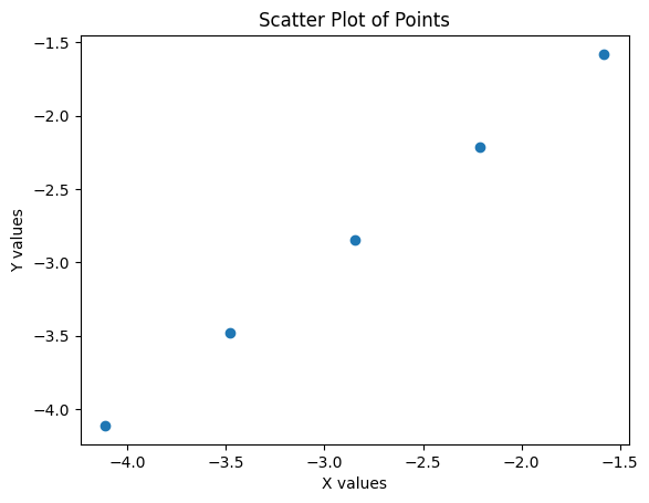
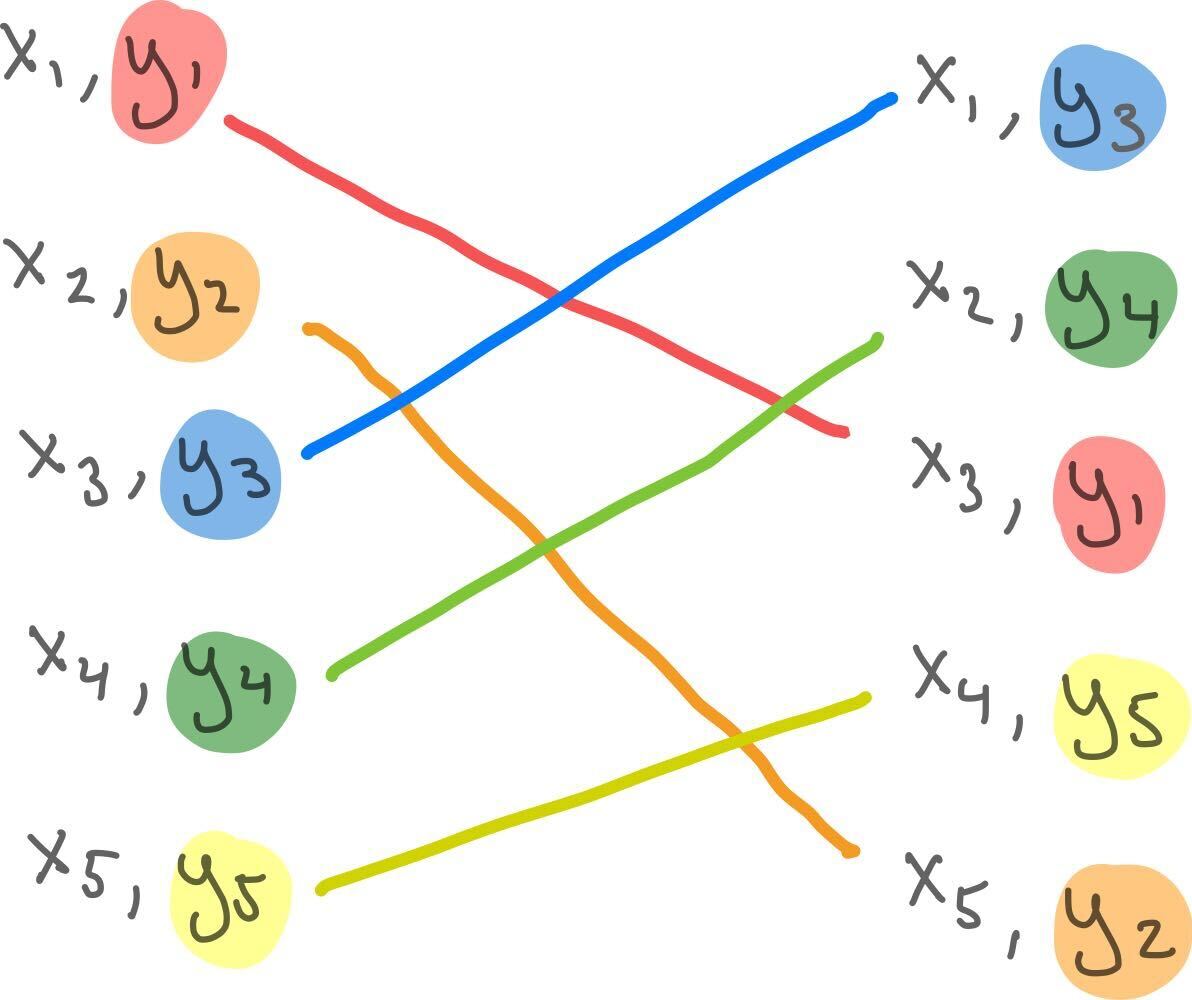
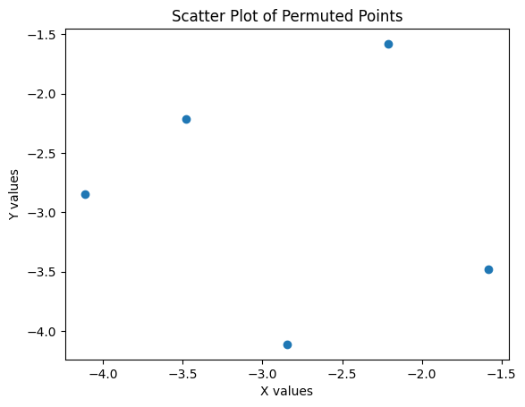
Now, what if we randomly shuffle or permute the $y_i$, so that they are matched to a random $x_j$?

There’s almost certainly no correlation now!

Null hypothesis based on shuffling#

Suppose we have computed $\hat R$ from our data. We want to know if $\hat R$ reflects an actual trend, or if it is just noise.

Null hypothesis: the pairs $(x_i,y_i)$ are paired up totally randomly.

Question: Why is this null hypothesis saying that there is no real correlation?
Question: In plain English, what is the $p$-value of $\hat{R}$?

The null is saying there is no real correlation because if the pairing of $x_i$ and $y_i$ is arbitrary/random, there would almost certainly not be a linear relationship.
The $p$-value is the chance that you’d get this value of $\hat{R}$, or a more extreme one, if the data were paired up by randomly shuffling.

Permutation test for correlation#

Suppose we have computed $\hat R$ from our data. We want to know if $\hat R$ reflects an actual trend, or if it is just noise.

Null hypothesis: the pairs $(x_i,y_i)$ are paired up totally randomly.

$p$-value: the chance that you’d get this value of $\hat{R}$, or a more extreme one, if the data were paired up by randomly shuffling.

We’ll compute the $p$-value using a Permutation test, a test based on simulation:

Do some large number $T$ of repetitions of the following experiment:

a. Randomly permute/shuffle the $y_i$ so that each is paired with some random $x_j$

b. Compute and record the correlation coefficient for the shuffled dataset
Make a histogram of the correlation coefficient values for all $T$ trials.
Decide the $p$-value for $\hat R$ based on how extreme it is relative to the histogram:
- If $\hat R$ is positive, the $p$-value for $\hat R$ is the fraction of histogram values larger than $\hat R$ (or $1/T$, if none are larger).
- If $\hat R$ is negative, the $p$-value for $\hat R$ is the fraction of histogram values smaller than $\hat R$ (or $1/T$, if none are smaller).

The penguins#

In Lecture 15, we computed a correlation coefficient of $\hat R = 0.67$ for Gentoo Penguin body mass vs. beak length.

What is the $p$-value?

I ran a simulation with $T = 10,000$ random permutations of the $y_i$, and computed the correlation coefficient each time.

Below is a histogram of the $T$ correlation coefficients for the random permutations.

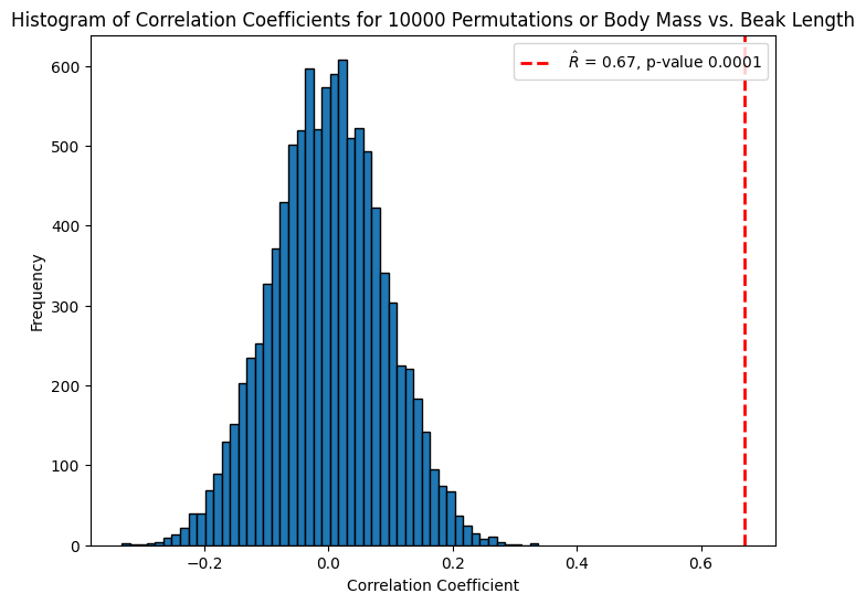
Using the permutation test, the $p$-value is at most $.0001$:

We conclude that $\hat R$ is statistically significant at level $\alpha = 0.05$ (or smaller).

GDP in 1960 vs. 2000#

In Lecture 15 we also computed the correlation coefficient for the GDP of countries in 1960 vs. 2000.

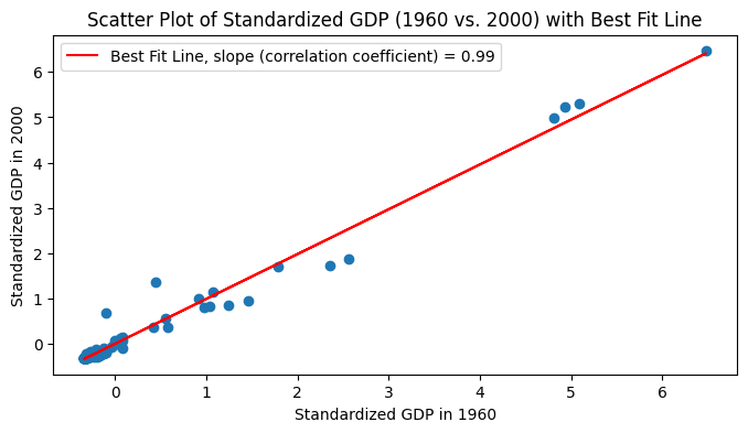
We can do a permutation test to check if this value of $\hat R$ is statistically significant.

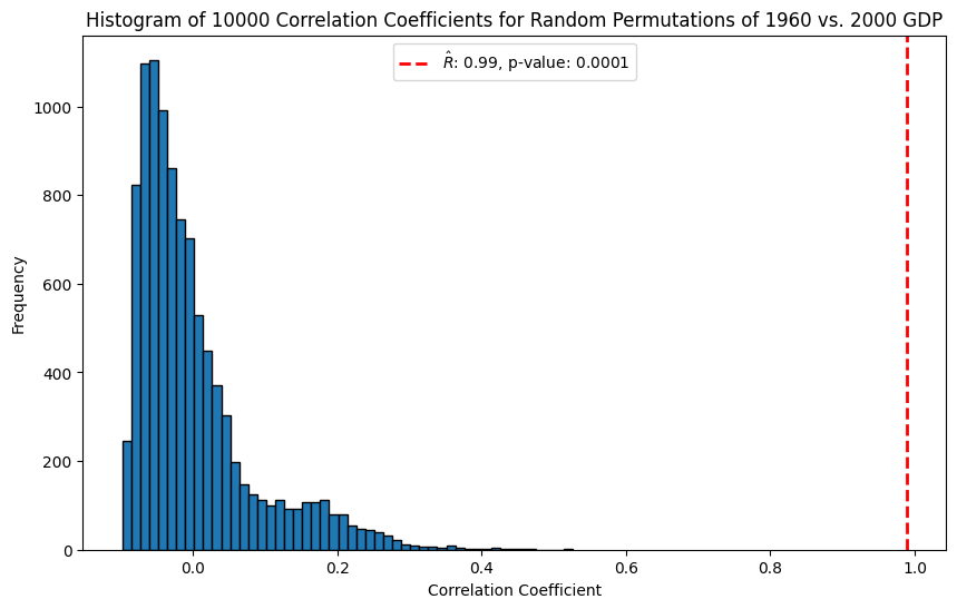
P-value for GDP correlation#

For $T = 10,000$ permutations, the $p$-value is for the correlation coefficient of 1960 vs. 2000 GDP is $1/10,000$:

Are nerds lonelier?#

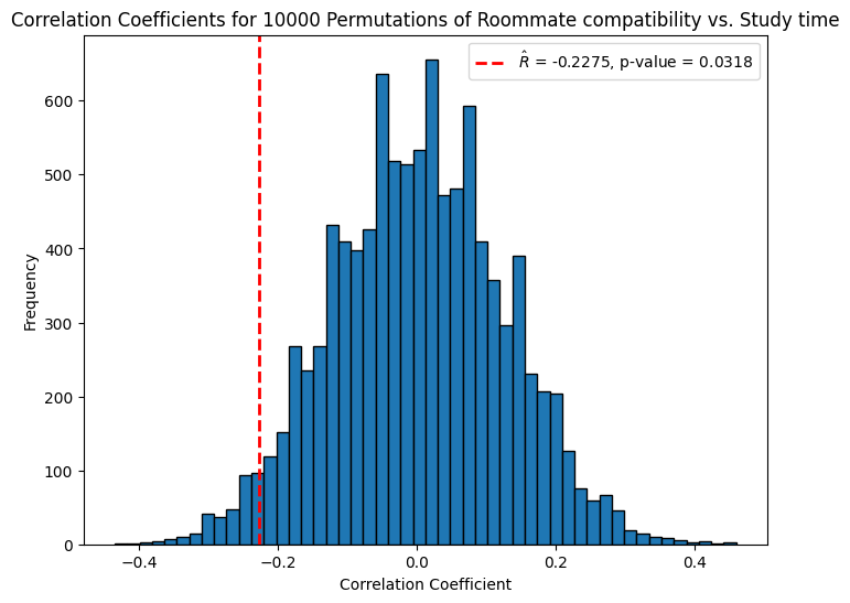
If we look at data from the course survey, we see a somewhat negative correlation between time spent studying and roommate compatibility. $\hat R \approx -.2$

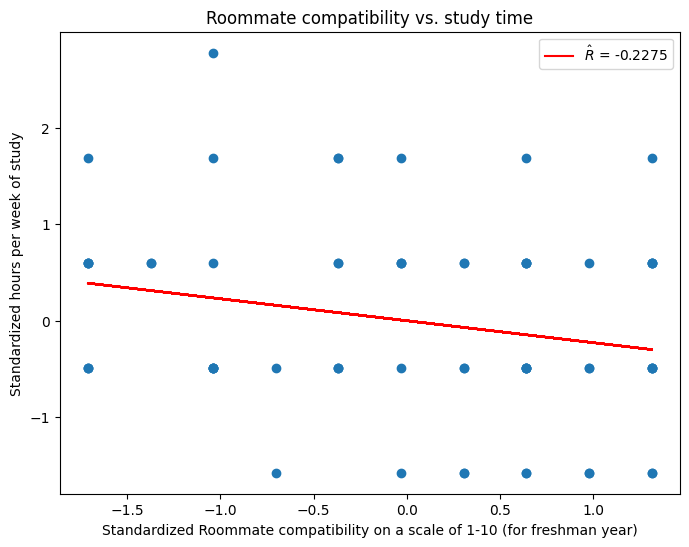
$p$-value for lonely nerds?#

Via simulation, for a $T = 10,000$-trial permutation test, we verify that the $p$-value is $\approx 0.03$, small enough that the trend is statistically significant at level $\alpha = 0.05$:

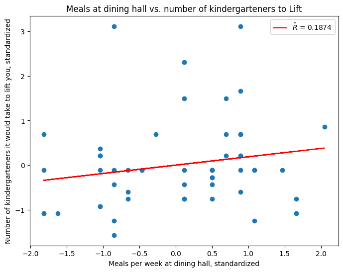
Are frequent diners too heavy for kindergarteners?#

We also see a positive correlation between the number of meals eaten at the dining hall each week and the number of (self-reported) kindergarteners it would take to lift you, $\hat R \approx 0.2$.

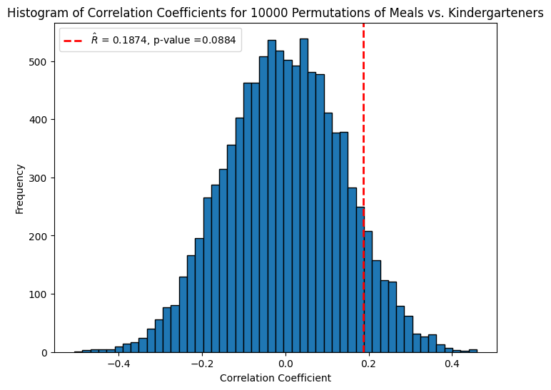
$p$-value for meals and kindergarteners#

Via simulation, we see that this $\hat R$ is not statistically significant at level $\alpha = 0.05$, $p$-value $\approx 0.08$.

Variability#

We computed $\hat R_n$. But what about its variability?

Is $\hat R_n$ being influenced by outliers?
If I had a slightly different sample, would my value of $\hat R_n$ be dramatically different?

The permutation-test $p$-values only give us a sense of statistical significance of a correlation:

we can see how extreme $\hat R_n$ is relative to a random shuffling of the data (no correlation)
we cannot see how $\hat R_n$ would vary if we had a different sample from data with the same type of associative relationship.

How much variability in lonely nerds?#

The lonely nerd trend from the course survey was statistically significant.

However, what is the variability like?

Would the value of $\hat R$ changed to a (smaller or larger) negative value if we had sampled differently?
How much smaller or larger?

Estimating variability with simulation#

We can use simulation to estimate variability too.

The best case scenario would be, if we have access to new samples from our population, just collect more samples and compute a fresh correlation coefficient a bunch of times.
But what if we don’t have access to new samples?

The following approach is called the bootstrap:

Start with our dataset $(x_1,y_1),\ldots,(x_n,y_n)$.
For some large number of trials $T$:

a. Sample $n$ pairs independently with replacement from the dataset: $$(x_{i_1},y_{i_1}),\ldots,(x_{i_n},y_{i_n})$$

b. Compute and record the correlation coefficient of these pairs.
Form a histogram of the correlation coefficients from all $T$ trials.
- To get a $1-\alpha$ confidence-interval around $\hat R_n$, choose the interval around $\hat R_n$ which contains $1-\alpha$ fraction of the results from the $T$ trials.

The Bootstrap#

To get a sense of the variability of $\hat R_n$:

Start with our dataset $(x_1,y_1),\ldots,(x_n,y_n)$.
For some large number of trials $T$:

a. Sample $n$ pairs independently with replacement from the dataset: $$(x_{i_1},y_{i_1}),\ldots,(x_{i_n},y_{i_n})$$

b. Compute and record the correlation coefficient of these pairs.
Form a histogram of the correlation coefficients from all $T$ trials.

Question: why could this simulation give us a good sense of variability? Will it account for outliers?

There’s a reasonable chance that we’ll avoid any specific outlier in a trial when we sample with replacement: $$\Pr[\text{avoid i }] = (1-\frac{1}{n})^n \approx e^{-1} \approx \frac{1}{3} \text{ when }n\text{ large.}$$
If we take a $2/3 \approx 66\%$ or larger confidence interval, it will likely contain the correlation coefficients from trial runs which avoid that outlier.

Question: will this always give us a good idea of the variability of $\hat R_n$?

Not necessarily; our sample could just be really weird.
A large enough sample probably reflects the population well enough that it should work pretty well. You can prove that this works with high probability when $n$ is sufficiently large enough.

Simulation for variability in loneliness of nerds#

If we do a bootstrap simulation with $T= 10,000$ trials, we can see that the confidence interval around $\hat R$ is quite large, almost (but not quite) containing $0$:

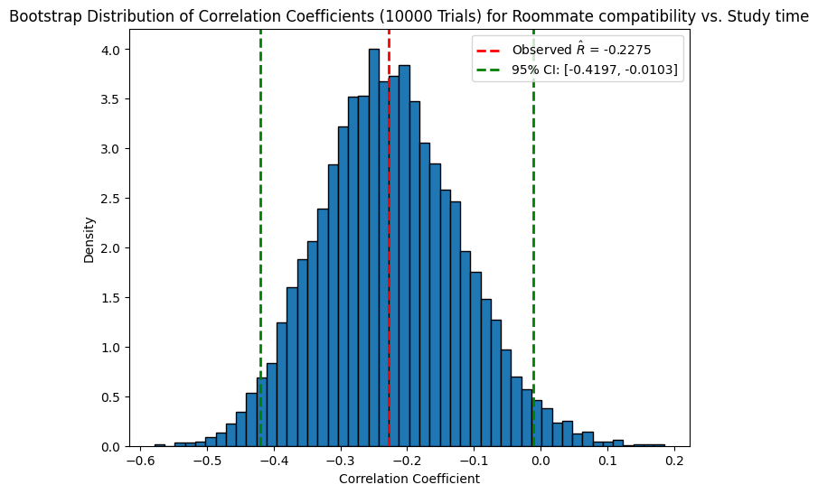
This gives us some sense of the variability of $\hat R_n$.

Question: Are we sure this confidence interval is accurate for the population distribution of all Stanford students?

No. Our class (and the people who completed the course survey) might be a biased sample. But this does give a sense of variability within our class.

Correlation is not causation!#

Even though we can test for the statistical significance of a correlation, we do not know if this is a sign of causality.

If our $(x_i,y_i)$ pairs are observational, we don’t know if: a. $x_i$ causes $y_i$ b. $y_i$ causes $x_i$ c. both are caused by some unseen variable $z_i$
In medicine and other scientific research, this happens all the time:
- For example, $x_i =$ how much fiber you eat, $y_i =$ cholesterol levels
- We may observe a negative correlation between these variables a. Does a healthy diet cause low cholesterol? b. Are people who eat healthy also more likely to exercise, thereby controlling their cholesterol? (The unseen variable $z_i =$ exercise)
Next week, experimental design and randomized control trials.

Recap#

Testing for correlation
- Using simulation: permutation tests
Variability of correlation
- Using simulation: “the bootstrap”