Lecture 16: Sample size matters

Lecture 16: Sample size matters#

STATS 60 / STATS 160 / PSYCH 10

Concepts and Learning Goals:

Estimating an unknown quantity by sampling
Larger sample improves accuracy
Population vs. sample distribution
Quantifying how accuracy improves with sample size
- standard deviation of the sample mean

Welcome to Unit 4: Correlation and Experiments!#

A burning question#

You want to know what fraction of people on campus think that a hot dog is a type of sandwich; call this unknown fraction $\mu$.

The population is large enough that you cannot afford to ask each person—it’s too time consuming, and too hard to ensure you really asked everyone.

What do you do?

The cube rule of food. Image credit: [wikihow

Estimating from a sample#

You estimate the fraction $\mu$ using a random sample!

Sample a uniformly random subset of $n$ people (with vs. without replacement doesn’t really matter if the population is large enough)
- Suppose $m$ out of $n$ sampled think a hot dog is a sandwich.
You take $\hat{\mu_n} = \frac{m}{n}$ as an estimate for $\mu$.

Question: Can you model this probabilistically with either a bag of marbles or with coinflips?

Question: Are we guaranteed that $\hat{\mu_n} = \mu$? Why?

How good is our estimate?#

Our poll is basically an experiment whose goal is to measure $\mu$.

Our estimate $\hat{\mu_n}$ is a random, noisy measurement of $\mu$.
The value of $\hat\mu_n$ depends on the sample. If we repeat the experiment, we could get a different value of $\hat{\mu_n}$.
It’s important for us to know if we can trust our estimate.
We can use probability (modeling with coinflips) to calculate, directly, the probability that $\hat{\mu_n}$ is far from $\mu$.
We can also approximate this probability in a smarter way, using a Normal approximation. More on Wednesday.

Another scenario#

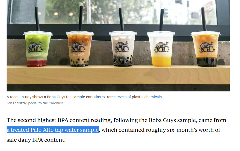
We want to determine the concentration of microplastics in Palo Alto tap water.

The concentration of microplastics is a fixed quantity, $\mu$.

How can we estimate $\mu$? Do an experiment!

We take $n$ independent water samples, measure the concentration of microplastics in each, and produce a set of measurements $x_1,\ldots,x_n$.
We estimate $\mu$ using the sample mean, $\hat{\mu_n} = \bar{x}$.

From an article in the SF chronicle.

How accurate is our estimate $\hat{\mu_n}$?

The estimate is random. If we repeat our experiment, we could get a different value of $\hat{\mu_n}$.
Can we compute the probability that $|\hat{\mu_n} - \mu|$ is big?
- In this case, it is not clear how to model this scenario with coins or marbles; we don’t know how the error of our measurements behaves.
We can still approximate this probability using a Normal approximation! More on Wednesday.

Size matters#

Before we get into understanding the probability that our estimate is accurate, let’s make one thing clear: Sample size matters.

Question: What do you expect to happen to our estimate $\hat{\mu_n}$ as $n$ gets larger?

As $n$ gets larger, we expect that our estimate $\hat{\mu_n}$ is more accurate.

Since $\hat{\mu_n}$ is random, there is always some chance it will be inaccurate. But as our sample size increases, the chance of $\hat{\mu_n}$ being accurate increases.

DIY poll#

From the class survey, we know $\mu = 40\%$ of the class believes a hot dog is a sandwich.

What if we try to estimate $\mu = .4$ from samples? Let’s see how the variability of $\hat{\mu_n}$ behaves as we increase the sample size $n$.

$\hat{\mu_n}$ is random. To understand what the distribution of $\hat{\mu_n}$ is as we vary $n$, we’ll do the following experiment:

For each $n$ in $\{2,4,8,16,32,64\}$:

We’ll conduct $50,000$ polls, each of $n$ students from our class.

a. Each of the $50,000$ polls produces $n$ responses.

b. We’ll compute a separate estimate $\hat{\mu_n}$ based on each poll

c. The $\hat{\mu_n}$’s form a dataset with $50,000$ samples.

d. We’ll plot the histogram of the dataset.

But we’ll simulate it with some code, to save time :)

import matplotlib.pyplot as plt
import random
T = 50000
mu = 43/107
Class = [1] * 43 + [0] * (107 - 43) # Make a list of "students" in the class; 1's are hot dog = sandwich people
Estimates = [0]*T


def trial(n):
    for t in range(T): # Run T independent polls
        X = random.sample(Class,n) # Survey n students each time
        Estimates[t] = sum(X)/n    # Record Q_n

    if n > 15:
        numbins = 12
    else:
        numbins = 15

    plt.hist(Estimates, bins=10) # Plot a histogram of the data 
    plt.xlabel('Estimate of $\mu$')
    plt.title('Variability in estimate of $\mu$, n ='+str(n))
    plt.axvline(x=mu, color='red', linestyle='--', linewidth=1)
    plt.xlim(0,1)
    plt.show()

<>:20: SyntaxWarning: invalid escape sequence '\m'
<>:21: SyntaxWarning: invalid escape sequence '\m'
<>:20: SyntaxWarning: invalid escape sequence '\m'
<>:21: SyntaxWarning: invalid escape sequence '\m'
/tmp/ipykernel_182615/870793613.py:20: SyntaxWarning: invalid escape sequence '\m'
  plt.xlabel('Estimate of $\mu$')
/tmp/ipykernel_182615/870793613.py:21: SyntaxWarning: invalid escape sequence '\m'
  plt.title('Variability in estimate of $\mu$, n ='+str(n))

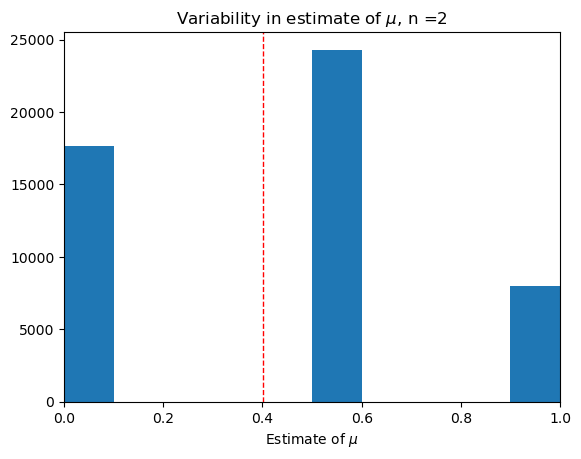
Smallest sample, $n = 2$.#

trial(2)

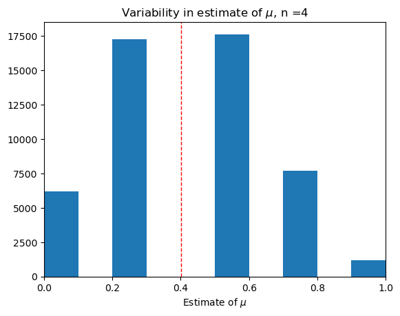
../_images/232ffafbab5ff687db73265cfbad03492c765eeeca039973d26d4eb9165dfd39.png

Small sample, $n = 4$.#

trial(4)

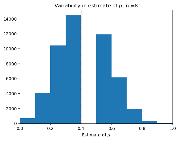
../_images/b40325f21705bc6ceadfb75a96148b5c5840ac36a52b2cc13a6f60748fecd6bb.png

Medium-small sample, $n=8$.#

trial(8)

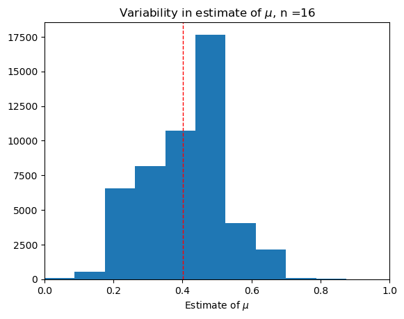
../_images/1431c286a222d06f42e32b6be500f1b35fbb477f2cfee9312807de7a79c1e8f7.png

Medium sample, $n = 16$.#

trial(16)

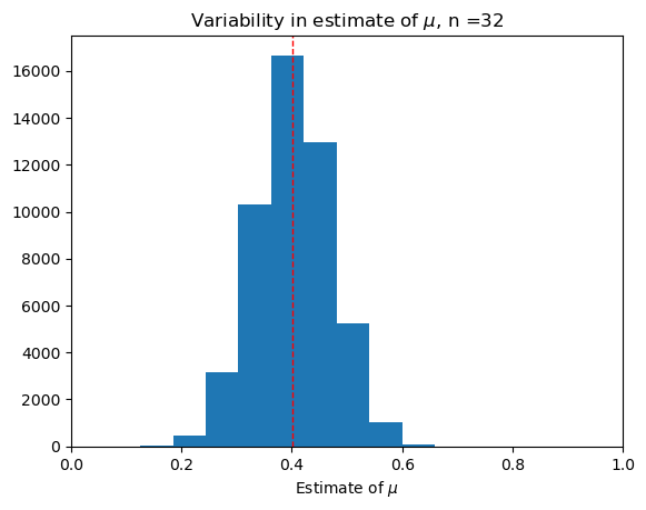
../_images/2709708fa5c2495234b7f9db774f3ffa49e59e483d2579679ce06cc921d8ebc6.png

Largeish sample, $n = 32$.#

trial(32)

../_images/c18f6a155af6eb433f48d192e0ee89ca52e58f418143f303ddd1427426e394d7.png

Large sample, $n = 64$#

trial(64)

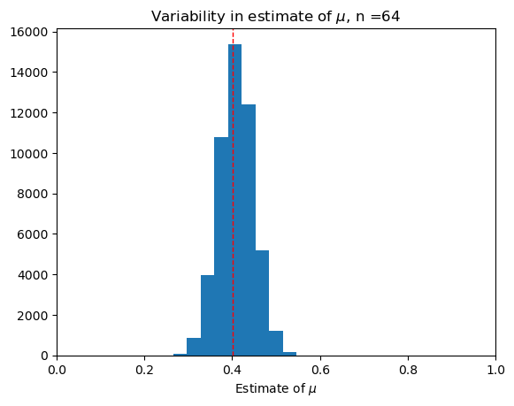
../_images/406672175abae4dfe3736d4fe2d83bc4051232658f1145f9e0f48a33ac1cb2df.png

What do you notice?#

Question: As we increase $n$, what do you notice about:

The variability of the dataset of our estimates $\hat{\mu}_n$?
The shape of the histogram?

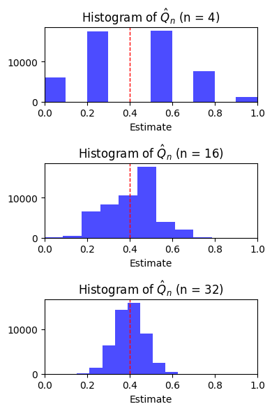
Larger sample size leads to decreased variability and increased accuracy of $\hat{\mu_n}$—it is more likely to be close to $\mu$.
The shape of the histogram looks more and more like an upside down bell.

We’ll focus on 1 today, return to 2 on Wednesday.

Bigger samples are better#

The tl;dr of this lecture is that sample size matters, and bigger is better.

A larger sample size leads to a more accurate estimate.

But now, we want to quantify how much more accurate the estimate becomes as the sample size increases.

For that, we formalize the concept of the population vs. the sample.

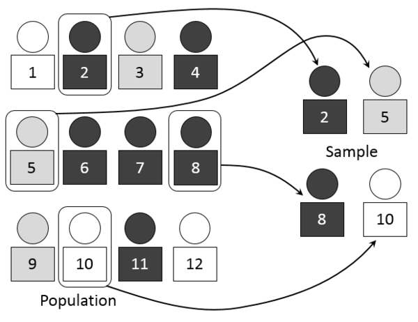
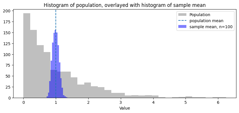
Population vs. sample#

Our experiments are all versions of the following meta:

There is variable $x$ which describes members of a “population”. Our goal is to estimate the population mean, $\mu$.
We take $n$ independent samples from the population, forming a sample dataset $$x_1,\ldots, x_n.$$
We form an estimate of $\mu$ using the sample mean $$\hat{\mu_n} = \frac{x_1+\cdots+x_n}{n}.$$

The sample mean is a random variable; its value depends on the randomness of our sample.

Our hope is that it is usually close to $\mu$.

Hotdog poll as “population vs. sample”#

We conduct a poll to figure out what fraction of Stanford students think that a hot dog is a sandwich.

The “population” is the $N$ students on campus.
There is a variable $x$ which describes members of a “population”:
- For each student, the variable $x$ takes value $1$ if the student thinks a hot dog is a sandwich, and $0$ otherwise.
- The population mean, $\mu$, is exactly the fraction of students who think a hot dog is a sandwich: $\mu = \frac{\sum x}{N}$
We take $n$ independent samples from the population, forming a dataset $$x_1,\ldots, x_n.$$
- Each student’s yes/no answer can be recorded as $x_i = 1$ if the student said yes, $x_i = 0$ if they said no.
We estimate $\mu$ using the sample mean $\hat{\mu_n} = \frac{x_1+\cdots+x_n}{n}$.

Microplastics as “population vs. sample”#

We take $n$ different measurements of microplastics concentration in Palo Alto tapwater, and take the sample mean to estimate the true concentration $\mu$.

The “population” is all possible water samples.
There is a variable $x$ which describes members of a “population”:
- In this experiment, the variable $x$ is the concentration of microplastics in particular water sample.
- The population mean, $\mu$, is the average concentration of microplastics in a water sample.
We take $n$ independent samples from the population, forming a dataset $$x_1,\ldots, x_n.$$
- Each water samples gives us a measurement $x_i$, the concentration of microplastics in that particular water sample.
We estimate $\mu$ using the sample mean $\hat{\mu_n} = \frac{x_1+\cdots+x_n}{n}$.

Now you try#

A medical researcher has come up with a new drug. The drug has a side effect: a headache that lasts anywhere from $0$ to $48$ hours. The researcher wants to determine what the average duration of the headache.

The researcher recruits a group of $n$ random sick patients, gives them all the drug, records the length of each of their headaches, and calculates the sample mean as an estimate of the average duration.

What is the population?
What is the variable $x$ that describes members of the “population”? What is the population mean $\mu$?
What are the samples?

Statistics of the sample vs. the population#

Suppose the population mean for the variable $x$ is $\mu$ and the population standard deviation is $\sigma_x$.

The sample mean $\hat \mu_n$ is a random variable.

Different samples could lead to different values of $\hat\mu_n$.

Assuming our $n$ samples are independent and uniform,

The expectation of the sample mean is equal to the population mean, $$\mathbb{E}[\hat\mu_n] = \mu.$$
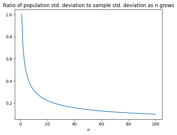
The standard deviation of the sample mean is $$\frac{\sigma_x}{\sqrt{n}}.$$
- That’s a factor $\frac{1}{\sqrt{n}}$ smaller than the standard deviation of $x$!

Quantifying “bigger is better”: As $n$ grows, the standard deviation of the sample mean $\hat{\mu}_n$ decreases!

Larger samples give more accurate estimates#

A large sample size reduces the standard deviation of the sample mean.

This is just a feature of the distribution of $\hat{\mu_n}$—what does it mean for accuracy?

The error $|\hat{\mu_n} - \mu|$ will usually be within a few multiples of the sample standard deviation $\frac{\sigma_x}{\sqrt{n}}$.

(As we discussed in lectures 14&15, this is guaranteed by something called Chebyshev’s inequality).

So to get $10$ times more accurate, it’s enough to increase $n$ by a factor of 100: $\sqrt{100} = 10$.

This plot gives a sense of how much more accurate it is to take a sample of size vs. a sample of size .

We’ll get more precise on Wednesday.

Recap#

We introduced the strategy of estimating an unknown feature of a population by random sampling.
We introduced the paradigm of the population vs. sample mean.
Sample size matters! Bigger is better.
The sample standard deviation is a $\frac{1}{\sqrt{n}}$ factor smaller than the population standard deviation.